Partial Generalized Probability Weighted Moments for Exponentiated Exponential Distribution

Partial Generalized Probability Weighted Moments

for Exponentiated Exponential Distribution

Neema Mohamed El Haroun Institute of Statistical Research Mathematical Statistics Department Cairo University, Egypt

[email protected]

Abstract

The generalized probability weighted moments are widely used in hydrology for estimating parameters of flood distributions from complete sample. The method of partial generalized probability weighted moments was used to estimate the parameters of distributions from censored sample. This article offers new method called partial generalized probability weighted moments (PGPWMs) for the analysis of censored data. The method of PGPWMs is an extended class from partial generalized probability weighted moments. To illustrate the new method, estimation of the unknown parameters from exponentiated exponential distribution based on doubly censored sample is considered. PGPWMs estimators for right and left censored samples are obtained as special cases. Simulation study is conducted to investigate performance of estimates for exponentiated exponential distribution. Comparison between estimators is made through simulation via their biases and mean square errors. An illustration with real data is provided.

Keywords: Generalized Probability Weighted Moments, Partial Probability Weighted Moments, Partial generalized Probability Weighted Moments, Generalized Exponential Distribution, Censored Samples.

1. Introduction

Gupta and Kundu (1999), introduced the generalized exponential distribution which, also known as exponentiated exponential (EE) distribution. It is observed that the EE distribution can be considered for situation where a skewed distribution for a non- negative random variable is needed. Also, it is observed that it can use quite effectively to analyze lifetime data in place of gamma, Weibull and log-normal distributions.

The probability density function of the two parameter EE distributions given by;



x; ,







1e



1e , , ,x0

f    x  x  

The corresponding cumulative distribution function is given by:



x; ,







1e



, , ,x0

F   x    (1)

The initial idea of PPWMs was to remove the smaller observations from the process of fitting the distribution because such observations are of little interest in flood frequency analysis and such observations can a nuisance to the fitting process. The method is computationally simple, robust and possesses the same merit as the original method of probability weighted moments.

Zafirakou-Koulouris et al (1998) introduced the evaluation of L- moments for a left censored observation from PPWMs. Deng and Pandey (2009) presented a new distribution for estimating quantile function of a non-negative random variable using a censored sample of data, which is based on the principle of partial maximum entropy in which PPWMs are used as constraints.

This article presents new method which is called partial generalized probability weighted moments for estimating the unknown parameters of distributions from censored samples. The PGPWMs will be used to estimate unknown parameters of EE distribution under doubly censored samples. Then, the PGPWMs estimators of the unknown parameters from left and right censored samples will be obtained as special cases. At the same time, the generalized probability weighted moments can be obtained as the special case from PGPWMs. To illustrate the properties of the new estimators, an extensive numerical study will be performed. Analysis of a real data set has been performed.

This article is organized as follows. In Section 2, the definition of PGPWMs and their sample estimators from doubly, right, and left censored samples is introduced. Section 3 discusses the PGPWMs method of estimation for the EE distribution from doubly, left and right censored samples. A simulation study is performed to investigate the properties of the new estimators from censored samples with two special cases in Section 4. Real data example is given in Section 5. Finally, the conclusions are included in Section 6. Tables and some Figures are included in the appendix.

2. The PGPWMs and Their Sample Estimators

The generalized probability weighted moments (GPWMs) were introduced by Rasmussen (2001) as a tool for estimating the parameters of probability distribution, for complete sample, expressible in inverse form. The GPWMs can be defined as



 





p u v



v u

p E X F X F X

M _{, ,}  ( ) 1 ( ) 





x

 

F



pFu



1F



vdF

1

0

, (2)

whereX is a random variable and F(x) is cumulative distribution function.

We introduce the method of PGPWMs as an extension class of GPWMs and PPWMs methods. The general form of PGPWMs with double bound censoring for the random variable X is defined as follows:

v u p

W , ,





 





v u

p

X F X

F X

E ( ) 1 ( )





x

 

F



Fu



F



vdF

d

c

p _

where, p1, u _and v to be real values (i.e. exponents uand v of the PGPWMs can be ratio or integers). Also, cF(x₀₁) and d F(x₀₂), x₀₁ and x₀₂ are lower and upper

bound censoring respectively; Therefore, forp1, andv0, W_p,r,s becomes;







u



u E X F X

W_{1, ,0}  ( )



x

 

F



FudF

d

c



 , (4)

It is noted when d 1 and the lower bound c0then the PGPWMs with double bound censoring is reduced to GPWMs in complete samples as defined in (2).

The PGPWMs with lower bound (left) censoring, denoted by LW1,u,0, can be obtained as a special case from (4)by putting d 1.Therefore, the general form of PGPWMs with left censoring for the random variable X takes the following form







u



u E X F X

LW1, ,0  ( )



x

 

F



F dF

u

c



 1 . (5)

The PGPWMs with upper bound (right) censoring, denoted by RW_1,u,0, can be defined as a special case from (4) by putting c0.Therefore, the general form of PGPWMs with right censoring for the random variable X takes the following form







u



u E X F X

RW_{1, ,0}  ( )



x

 

F



FudF

d



 0

. (6)

Let x_{ 1} ,x_{ 2} ,...,x_{ n} be a random sample of size n from the distribution functionF

 

X , and x_{ 1} x_{ 2} ,... x_{ n} be the corresponding ordered sample. According to Hosking (1986), the estimates of W1,u,0,LW1,u,0 and RW1,u,0is defined as the following

. 35 . 0 ˆ

1 ) ( 0

, , 1

u n

i i u

n i x

W 

  

  







(7)

. 35 . 0 ˆ

1 ) ( 0

, , 1

u n

i i u

n i x W

L 

  

  







(8)

. 35 . 0 ˆ

1 ) ( 0

, , 1

u n

i i u

n i x W

R 

  

  







(9)

Note that, the PGPWM estimators with doubly, left or right censoring is obtained by equating the theoretical PGPWM with the corresponding sample PGPWM.

3. PGPWMs Estimation of the EE

(3.1) PGPWMs Estimation of the EE from Doubly Censored Sample

The theoretical PGPWMs with double bound censored, W_1,u,0 for the EE distribution can be found from (4) after setting u u₁and uu₂as the following;



0 , , 1u₁

W



x

 

F



FudF

d c 1





          1 1 1 1 ] ) 1 ( [

1 1 1

j u j u j u j j c d     (10)  0 , , 1u2

W



x

 

F



Fu dF

d c 2





          1 2 1 1 ] ) 1 ( [

1 2 2

j u j u j u j j c d     (11)

From Equations (10) and (11), the two parameters,  and , can be expressed as follows: 0 , , 1 1 1 1 1 1 1 1 ] ) 1 ( [ u j u j u j W u j j c d



             

. (12)

0 ] ) 1 ( [ ] ) 1 ( [ 1 2 1 1 0 , , 1 1 1 1 1 0 , , 1 2 2 1 1 1 2        





            j u j u j u j u j u j u u j j c d W u j j c d W      

. (13)

The PGPWMs estimators of  _and  _{from doubly censored samples, can be obtained by} solving equations (12) and (13) in terms of and; where W1,u₁,0 and W1,u₂,0 are replaced

by their sample estimators, _{1, ,0} 1 ˆ

u

W and _{1, ,0} 2 ˆ

u

W given by Equation (7) by setting uu₁,u₂,

therefore 0 , , 1 1 1 1 ˆ 1 ˆ 1 1 1 ˆ ] ) 1 ˆ ( [ ˆ u j u j u j W u j j c d



             

. (14)

0 ] ) 1 ˆ ( [ ˆ ] ) 1 ˆ ( [ ˆ 1 2 1 ˆ 1 ˆ 0 , , 1 1 1 1 ˆ 1 ˆ 0 , , 1 2 2 1 1 1 2        





            j u j u j u j u j u j u u j j c d W u j j c d W      

, (15)

Some special cases can be obtained from the above the PGPWMs

1. For u₁ 0and u₂ 1, the PPWMs can be obtained from PGPWMs with doubly censored as obtained by Al-Khodary et al (2008).

2. For c0and d 1, the GPWMs can be obtained from PGPWMs with doubly censored as obtained by El Haroun (2009).

3. Foru₁ 0,u₂ 1, c0and d 1, the PWMs can be obtained from PGPWMs with doubly censored as obtained by Al-Khodary et al (2007).

(3.2) PGPWMs Estimation of the EE from Left Censored Sample

The theoretical PGPWMs with left bound censored, LW_1,u,0 for the EE distribution can be found from (5) after setting uu₁and u u₂as the following;



0 , , 1u₁

LW



x

 

F



Fu dF

c 1 1





        1 1 1 ] ) 1 ( 1 [ 1 1 j u j u j j c    (16)  0 , , 1u2

LW



x

 

F



Fu dF

c 2 1





        1 2 1 ] ) 1 ( 1 [ 1 2 j u j u j j c    (17)

From Equations (16) and (17), the two parameters,  and, can be expressed as follows:

0 , , 1 1 1 1 1 1 ] ) 1 ( 1 [ u j u j LW u j j c



          

. (18)

0 ] ) 1 ( 1 [ ] ) 1 ( 1 [ 1 2 1 0 , , 1 1 1 1 0 , , 1 2 1 1 2        





        j u j u j u j u u j j c LW u j j c LW    

. (19)

To compute the PGPWMs estimators of  _and , denoted by ˆ_{L and} ˆ_L, from left

censored samples, _{1, ,0} 1

u

LW and _{1, ,0} 2

u

LW are replaced by their sample estimators, _{1, ,0} 1 ˆ

u

W L

and LWˆ1,u₂,0 by setting u u1,u2 in Equation (8), hence

0 , , 1 1 1 1 ˆ 1 1 ˆ ] ) 1 ˆ ( 1 [ ˆ u j L u j L W L u j j c L



          

0 ] ) 1 ˆ ( 1 [ ˆ ] ) 1 ˆ ( 1 [ ˆ 1 2 1 ˆ 0 , , 1 1 1 1 ˆ 0 , , 1 2 1 1 2        





        j L u j u j L u j u u j j c W L u j j c W L L L     (21)

Solving numerically by iteration Equation (20) to obtain ˆ . Once the estimate of _L  is determined, an estimate of  is obtained by substitute ˆ in Equation (21). _L

(3.3) PGPWMs Estimation of the EE from Right Censored Sample

The theoretical PGPWMs with right bound censored, RW_1,u,0 for the EE distribution can be obtained from (6) after setting uu_{1 and} u u_{2 as the following}



0 , , 1u1

RW



x

 

F



Fu dF

d 1 0





       1 1 1 ] ) 1 ( [ 1 1 j u j u j j d    (22)  0 , , 1u₂

RW



x

 

F



Fu dF

d 2 0





       1 2 1 ] ) 1 ( [ 1 2 j u j u j j d    (23)

From Equations (22) and (23), the two parameters,  and , can be expressed as follows: 0 , , 1 1 1 1 1 1 ] ) 1 ( [ u j u j RW u j j d



         

. (24)

0 ] ) 1 ( [ ] ) 1 ( [ 1 2 1 0 , , 1 1 1 1 0 , , 1 2 1 1 2      





        j u j u j u j u u j j d RW u j j d RW    

. (25)

The PGPWMs estimators of  _and , denoted byˆ and _R ˆ , from right censored _R samples, can be obtained by solving Equations (24) and (25); where _{1, ,0}

1

u

RW and _{1, ,0} 2

u

RW

are replaced by their sample estimators, RWˆ1,u₁,0 and RWˆ1,u₂,0by setting uu1,u2, in

Equation (9) as follows

0 , , 1 1 1 1 ˆ 1 1 ˆ ] ) 1 ˆ ( [ ˆ u j R u j R W R u j j d R



         

. 0 ] ) 1 ˆ

( [ ˆ

] ) 1 ˆ

( [ ˆ

1

2 1 ˆ

0 , , 1 1

1 1 ˆ

0 , , 1

2

1 1

2 

  













  



 

j

R u j

u j

R u j

u

u j j

d W

R u

j j

d W

R

R R

 

 

(27)

A numerical procedure is required to estimate based on iterative technique. Thus the value of ˆ can be obtained by substituting the value of_R ˆ in Equation (27). _R

4.

Numerical Experiments and Discussions

An extensive numerical study is carried out to investigate the properties of the PGPWMs method of estimation for the EE distribution from censored samples. The investigated properties are biases and mean square error (MSE) of the PGPWMs estimators of the two parameters and . The simulation procedure can be summarized as the following steps:

Step (1): 1000 random sample, x₁,x₂,...,x_n, of sizes n = 15, 20, 25, 30, 35and 50 are generated from the EE distribution.

Step (2): The true parameter selected values for the shape parameter  are 0.5, 0.6, 0.7 with scale parameter1. Choosing the exponent values of PGPWMs as u₁ 0,0.1,0.5and u₂ 1,0.4,1.5. Levels of censoring are considered, namely c0.2 and d 0.8.

Step (3): For each combination of values of sample size n,  and , the parameters of distribution are estimated using three different estimation methods; PGPWMs with doubly, left and right censored samples.

Step (4): PGPWMs of the unknown parameter  for EE distribution with doubly censored samples are obtained by solving numerically the non-linear Equation (15). The estimate of the scale parameteris obtained by substituting the value of ˆ in (14).

Step (5): Based on left censored samples, PGPWMs of the shape parameter for EE distribution is obtained by solving iteratively the non-linear Equation (21). Hence the ˆ is obtained by substituting the value of _L ˆ_Lin (20)

Step (6): Based on right censored samples, PGPWMs of the shape parameter  for EE distribution is obtained by solving numerically the non-linear Equation (27). To compute ˆ , substitute_R ˆ_Rin (26)

Step (7): PPWMs estimators with doubly, left and right censored samples for for EE distribution is obtained by solving numerically the non-linear Equations (15),(21) and (27) after setting u1 0and u2 1. Then, the

estimates ofis obtained by substituting the estimate of in Equations (14), (20) and (26).

All simulation studies presented here are obtained via the MathCAD14 software. The MSE of the different estimators of  and  are reported in Tables (1-6) and described in Figures (1-18). From simulation study many observations can be made on the performance of PGPWMs estimators with doubly, left and right censored samples. These observations are summarized as follows:

1. It is observed from Tables (1),(2)and (3) that the MSE of estimators for decreases as the sample size increases. This indicate that PGPWMs based on doubly, left and right censoring provided consistent estimators for  [see Figures(1-9)]

2. It is observed from Tables (4),(5)and (6) that the MSE of estimators for decreases as the sample size increases. This indicates that PGPWMs with doubly, left and right censoring provided consistent estimators for [see Figures (10-18)]

3. When the exponents of PGPWMs u₁ and u₂decrease, the MSE of estimators for

 and decreases [see Figures (1-18) and Tables (1-5)]

4. Considering the MSE of the different estimators of  , it is clear from Tables (1) (2)and (3) that the PGPWMs under right censoring estimator has the minimum MSE in almost all of the cases followed by PGPWMs under doubly censoring and the PGPWMs under left censoring [see Figures(1-9)]

5. Considering the MSE of the different estimators of , it is clear from Tables (4), (5)and (6) that the PGPWMs under right censoring estimator has the minimum MSE in almost all of the cases followed by PGPWMs under doubly censoring and PGPWMs under left censoring [see Figures (10-18)].

5. Data Analysis

This section presents a real data set for illustrative purposes. Lawless (1982) provided real data, which represents the numberof million revolutions before failure for each of 23 ball bearings in a life test: 17.88, 28.92, 33.00, 41.52, 42.12, 45.60, 48.80, 51.84, 51.96, 54.12, 55.56, 67.80, 68.64, 68.64, 68.88, 84.12, 93.12, 98.64, 105.12, 105.84, 127.92, 128.04, and 173.40.

Data analysis is presented to illustrate different PGWMs estimators from doubly, left and right censored samples. The data set is carried out to investigate the properties of the PGPWMs method of estimation for the EE distribution. The investigated properties of estimators for the two parametersand are biases and MSEs. The results are displayed in Tables 7 and 8 and some observations are summarized as follows:

1. Considering the MSE of the estimator for  , it is clear from Table (7) that the PGPWMs under doubly censoring estimator has the minimum MSE in almost all of the cases considered for estimating follow it PGPWMs under right censoring and the final PGPWMs under left censoring.

6. Concluding Remarks

In this study, the method of PGPWMs is introduced as a new method for estimating the parameters of distribution from censored sample. This framework covers the methods; PWMs, PPWMs and GPWMs. The GPWMs can be obtained via PGPWMs by setting the lower bound c=0 and upper bound d=1. Also, the PPWMs can be obtained from PGPWMs by setting the exponents of methods uequal integer numbers. Finally, the PWMs can be obtained from PGPWMs by setting the exponents of methods uequal integer numbers and the lower and upper bound equal 0 and 1 respectively

The method of PGPWMs has been applied for estimating the unknown parameters of EE distribution from doubly censored sample. This method has two special cases the left and right censored samples. All methods have provided consistent estimators for shape and scale parameters of EE distribution in terms of MSE. Comparing the performance of estimators from doubly, left and right censored samples the PGPWMs with right censored have the smallest MSE.

References

1. Al-Khodary, E., Hassan, A., and Allam, S. (2007). Self-determinant probability weighted moments method for estimating the parameters of the generalized exponential distribution. Proceeding of the 19st Annual Conference Statistics and Computer Modeling in Human and Social Sciences, Faculty of Economics and Political Science, Cairo University. 19, 159-176.

2. Al-Khodary, E., Hassan, A., and Allam, S. (2008). Double Censoring Partial Probability Weighted Moments Estimation of the Generalized Exponential Distribution, InterStat, pp. 1–24.

3. Deng, J. and Pandey, M.D. (2009). Using Partial Probability Weighted Moments and Partial Maximum entropy to estimate Quantiles from Censored Samples

Probabilistic Engineering Mechanics, 24, 407- 417.

4. ElHaroun, N.M. (2009). Generalized Probability Weighted Moments Estimators for Some Distributions. M.Sc. Thesis, Cairo University.

5. Hosking, J. R. M. (1986). The Theory of Probability Weighted Moments. Research Report RC 12210, IBM Research Division, Yorktown Heights, NY.

6. Gupta, R.D. and Kundu, D. (1999). Generalized exponential distributions,

Australian and New Zealand Journal of Statistics, 41(2), 173-188.

7. Lawless, J. F. (1982). Statistical Models and Methods for Lifetime Data, John Wiley & Sons, New York

8. Rasmussen, P. (2001). Generalized Probability Weighted Moment: Application to the Generalized Pareto Distribution. Water Resources Research, 37, 6, 1745-1751.

9. Wang, Q.J. (1990a). Estimation of the GEV distribution from censored samples by method of partial probability weighted moments, Journal of Hydrology, 120

10. Wang, Q. J. (1990b). Unbiased estimation of probability weighted moments and partial probability weighted moments from systematic and historical flood information and their application to estimating the GEV distribution. Journal of Hydrology 120, 115–124.

11. Wang, Q. J. (1996). Using partial probability weighted moments to fit the extreme value distributions to censored samples. Water Resources Research, 32(6), 1767– 1771.

Appendix

Figure1: The MSE of ˆ,ˆ_L,ˆ_{Rwhen u1=0.1}

u2=0.4for =0.5

Figure2: The MSE of ˆ,ˆ_L,ˆ_{Rwhen u1=0.1,}

u2=0.4 for  =0.6

Figure3: The MSE of ˆ,ˆ_L,ˆ_{Rwhen u1=0.1,}

u2=0.4 for =0.7

Figure4: The MSE of ˆ,ˆ_L,ˆ_{Rwhen u1=0.5}

u2=1.5for  =0.5

Figure5: The MSE of ˆ,ˆ_L,ˆ_{Rwhen u1=0.5}

u2=1.5for  =0.6

Figure6: The MSE of ˆ,ˆ_L,ˆ_{Rwhen u1=0.5}

u2=1.5for  =07

10 20 30 40 50

0.2 0.4 0.6 0.8 1 1.2

MsE_D1

MsE_L1

MsE_R1

n

10 20 30 40 50

0 0.5 1 1.5

MsE_D2

MsE_L2

MsE_R2

n

10 20 30 40 50

0.4 0.6 0.8 1 1.2

MsE_D4

MsE_L4

MsE_R4

n

10 20 30 40 50

0 1 2 3

MsE_D6

MsE_L6

MsE_R6

n

10 20 30 40 50

0 0.5 1 1.5

MsE_D5

MsE_L5

MsE_R5

n

10 20 30 40 50

0 1 2 3

MsE_D3

MsE_L3

MsE_R3

Figure7: The MSE of ˆ,ˆ_L,ˆ_{Rwhen u1=0}

u2=1for =0.5

Figure8: The MSE of ˆ,ˆ_L,ˆ_{Rwhen u1=0}

u2=1for  =0.6

Figure10: The MSE of ˆ,ˆ_L,ˆ_{Rwhen u1=0.1}

u2=1 for  =0.5

Figure11: The MSE of ˆ,ˆ_L,ˆ_{Rwhen u1=0.1}

u2=1 for =0.6

Figure12: The MSE of ˆ,ˆ_L,ˆ_{Rwhen u1=0.1}

u2=1 for  =0.7 Figure9: The MSE of ˆ,ˆ_L,ˆ_{Rwhen u1=0}

u2=1for  =0.5

10 20 30 40 50

0.4 0.6 0.8 1 1.2

MsE_D7

MsE_L7

MsE_R7

n

10 20 30 40 50

0 0.5 1 1.5

MsE_D8

MsE_L8

MsE_R8

n

10 20 30 40 50

0 1 2 3

MsE_D9

MsE_L9

MsE_R9

n

10 20 30 40 50

0 0.5 1 1.5 2

MsE_D11

MsE_L11

MsE_R11

n

10 20 30 40 50

0 0.5 1 1.5 2 2.5

MsE_D12

MsE_L12

MsE_R12

n

10 20 30 40 50

0.4 0.6 0.8 1 1.2 1.4 1.6

MsE_D10

MsE_L10

MsE_R10

Figure13: The MSE of ˆ,ˆ_L,ˆ_{Rwhen u1=0.1}

u2=0.4 for  =0.5

Figure14: The MSE of ˆ,ˆ_L,ˆ_{Rwhen u1=0.1}

u2=0.4 for  =0.6

Figure16: The MSE of ˆ,ˆ_L,ˆ_{Rwhen u1=0.5}

u2=1.5 for  =0.5 Figure15: The MSE of ˆ,ˆ_L,ˆ_{Rwhen u1=0.1}

u2=0.4 for =0.7

Figure17: The MSE of ˆ,ˆ_L,ˆ_{Rwhen u1=0.5}

u2=1.5 for  =0.6

Figure18: The MSE of ˆ,ˆ_L,ˆ_{Rwhen u1=0.5}

u2=1.5 for  =0.7

10 20 30 40 50

0 0.5 1 1.5

MsE_D13

MsE_L13

MsE_R13

n

10 20 30 40 50

0 0.5 1 1.5 2

MsE_D14

MsE_L14

MsE_R14

n

10 20 30 40 50

0 0.5 1 1.5 2

MsE_D16

MsE_L16

MsE_R16

n

10 20 30 40 50

0 0.5 1 1.5 2

MsE_D17

MsE_L17

MsE_R17

n

10 20 30 40 50

0 0.5 1 1.5 2 2.5

MsE_D18

MsE_L18

MsE_R18

n

10 20 30 40 50

0 1 2 3

MsE_D15

MsE_L15

MsE_R15

Table 1: Mean, Bias and MSE of PGPWMs Parameter Estimators for EE distribution from Doubly, Left and Right Censoring for u1 0.5 and

5 . 1

2 

u

Sample size n

Properties of 

PGPWMs of ˆ LPPWMs of ˆ_L RPPWMs of ˆ_R



=0.5



=0.6



=0.7



=0.5



=0.6



=0.7



=0.5



=0.6



=0.7

15

Mean 0.277 0.349 0.425 0.137 0.281 0.464 0.290 0.369 0.436

Bias -0.723 -0.651 -0.575 -0.863 -0.719 -0.536 -0.710 -0.631 -0.564

MSE 0.644 0.637 0.664 1.078 1.466 2.581 0.614 0.582 0.725

20

Mean 0.296 0.417 0.489 0.078 0.196 0.458 0.318 0.440 0.519

Bias -0.704 -0.583 -0.511 -0.922 -0.804 -0.542 -0.682 -0.560 -0.481

MSE 0.625 0.598 0.662 1.034 1.369 2.683 0.586 0.517 0.537

25

Mean 0.316 0.437 0.555 0.077 0.136 0.278 0.340 0.439 0.571

Bias -0.684 -0.563 -0.445 -0.923 -0.864 -0.722 -0.660 -0.561 -0.429

MSE 0.606 0.574 0.627 1.061 1.292 2.053 0.561 0.508 0.494

30

Mean 0.348 0.489 0.601 0.058 0.102 0.265 0.361 0.505 0.597

Bias -0.652 -0.511 -0.399 -0.942 -0.898 -0.735 -0.639 -0.495 -0.403

MSE 0.570 0.555 0.626 1.063 1.240 2.172 0.532 0.456 0.484

35

Mean 0.388 0.490 0.601 0.018 0.069 0.144 0.407 0.525 0.617

Bias -0.612 -0.510 -0.399 -0.982 -0.931 -0.856 -0.593 -0.475 -0.383

MSE 0.540 0.521 0.627 1.004 1.172 1.625 0.489 0.433 0.464

50

Mean 0.405 0.533 0.688 0.003 0.024 0.098 0.442 0.544 0.724

Bias -0.595 -0.467 -0.312 -0.997 -0.976 -0.902 -0.558 -0.456 -0.276

MSE 0.519 0.482 0.579 1.003 1.074 1.482 0.462 0.400 0.389

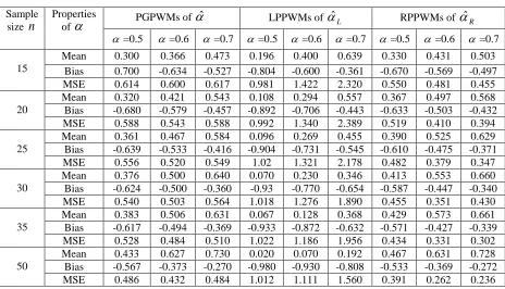
Table 2: Mean, Bias and MSE of PGPWMs Parameter Estimators for EE distribution from Doubly, Left and Right Censoring for u₁ 0.1 _and

4 . 0

2 

u

Sample size n

Properties

of  PGPWMs of ˆ LPPWMs of ˆL RPPWMs of ˆR

=0.5  =0.6 =0.7 =0.5  =0.6  =0.7  =0.5 =0.6 =0.7

15

Mean 0.300 0.366 0.473 0.196 0.400 0.639 0.330 0.431 0.503

Bias 0.700 -0.634 -0.527 -0.804 -0.600 -0.361 -0.670 -0.569 -0.497

MSE 0.614 0.600 0.617 0.981 1.422 2.320 0.550 0.481 0.455

20

Mean 0.320 0.421 0.543 0.108 0.294 0.557 0.367 0.497 0.568

Bias -0.680 -0.579 -0.457 -0.892 -0.706 -0.443 -0.633 -0.503 -0.432

MSE 0.588 0.543 0.588 0.992 1.340 2.389 0.519 0.410 0.394

25

Mean 0.361 0.467 0.584 0.096 0.269 0.455 0.390 0.525 0.629

Bias -0.639 -0.533 -0.416 -0.904 -0.731 -0.545 -0.610 -0.475 -0.371

MSE 0.556 0.520 0.549 1.02 1.321 2.178 0.482 0.379 0.347

30

Mean 0.376 0.500 0.640 0.070 0.230 0.346 0.413 0.553 0.660

Bias -0.624 -0.500 -0.360 -0.93 -0.770 -0.654 -0.587 -0.447 -0.340

MSE 0.540 0.503 0.564 1.018 1.276 1.890 0.455 0.351 0.430

35

Mean 0.383 0.506 0.631 0.067 0.128 0.368 0.429 0.573 0.661

Bias -0.617 -0.494 -0.369 -0.933 -0.872 -0.632 -0.571 -0.427 -0.339

MSE 0.528 0.484 0.510 1.022 1.186 1.956 0.434 0.331 0.302

50

Mean 0.433 0.627 0.730 0.020 0.070 0.192 0.467 0.631 0.728

Bias -0.567 -0.373 -0.270 -0.980 -0.930 -0.808 -0.533 -0.369 -0.272

Table 3: Mean, Bias and MSE of the PPWMs Parameter Estimators for EE distribution from Doubly, Left and Right Censoring when u1 0 and

1

2 

u

Sample size n

Properties of 

PGPWMs of ˆ LPPWMs of ˆ_L RPPWMs of ˆ_R

=0.5  =0.6  =0.7 =0.5 =0.6 =0.7 =0.5 =0.6  =0.7

15

Mean 0.298 0.387 0.508 0.197 0.352 0.524 0.330 0.409 0.519

Bias -0.702 -0.613 -0.492 -0.803 -0.648 -0.476 -0.670 -0.591 -0.481

MSE 0.619 0.593 0.650 1.022 1.337 2.316 0.557 0.506 0.473

20

Mean 0.326 0.423 0.543 0.103 0.268 0.430 0.367 0.468 0.552

Bias -0.674 -0.577 -0.457 -0.897 -0.732 -0.570 -0.633 -0.532 -0.448

MSE 0.589 0.561 0.618 1.011 1.372 2.276 0.515 0.448 0.432

25

Mean 0.358 0.485 0.599 0.079 0.185 0.455 0.388 0.503 0.604

Bias -0.642 -0.515 -0.401 -0.921 -0.815 -0.545 -0.612 -0.497 -0.396

MSE 0.559 0.521 0.609 1.024 1.233 2.374 0.488 0.413 0.388

30

Mean 0.366 0.506 0.610 0.043 0.130 0.322 0.409 0.546 0.644

Bias -0.634 -0.494 -0.390 -0.957 -0.817 -0.678 -0.591 -0.454 -0.356

MSE 0.553 0.515 0.572 1.007 1.183 1.941 0.470 0.378 0.358

35

Mean 0.389 0.525 0.653 0.026 0.148 0.346 0.431 0.565 0.675

Bias -0.611 -0.475 -0.347 -0.974 -0.852 -0.654 -0.569 -0.435 -0.325

MSE 0.525 0.491 0.542 1.004 1.251 2.180 0.441 0.351 0.331

50

Mean 0.417 0.547 0.736 0.008 0.067 0.142 0.456 0.627 0.72

Bias -0.583 -0.453 -0.264 -0.992 -0.933 -0.858 -0.544 -0.373 -0.280

MSE 0.503 0.469 0.515 1.007 1.123 1.480 0.416 0.301 0.273

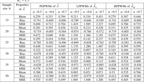
Table 4: Mean, Bias and MSE of PGPWMs Parameter Estimators for EE distribution from Doubly, Left and Right Censoring for u1 0.5 _and

5 . 1

2 

u Sample

size n

Properties

of  PGPWMs of 

ˆ _{LPPWMs of}

L

ˆ _{RPPWMs of}

R

ˆ

 =0.5 =0.6 =0.7 =0.5  =0.6 =0.7 =0.5 =0.6  =0.7

15

Mean 0.259 0.331 0.394 0.211 0.334 0.451 0.279 0.367 0.446

Bias -0.741 -0.669 -0.606 -0.789 -0.666 -0.549 -0.741 -0.669 -0.606

MSE 0.696 0.712 0.704 1.419 1.585 2.227 0.695 0.706 0.733

20

Mean 0.281 0.395 0.436 0.124 0.214 0.428 0.311 0.435 0.501

Bias -0.719 -0.605 -0.564 -0.874 -0.786 -0.572 -0.719 -0.605 -0.564

MSE 0.672 0.660 0.66 1.194 1.366 2.181 0.675 0.634 0.676

25

Mean 0.295 0.418 0.504 0.101 0.142 0.237 0.328 0.439 0.555

Bias -0.705 -0.582 -0.496 -0.899 -0.858 -0.763 -0.705 -0.582 -0.496

MSE 0.648 0.641 0.640 1.170 1.280 1.487 0.651 0.599 0.599

30

Mean 0.322 0.452 0.545 0.075 0.097 0.215 0.345 0.494 0.578

Bias -0.678 -0.548 -0.455 -0.925 -0.903 -0.785 -0.678 -0.548 -0.455

MSE 0.615 0.589 0.588 1.153 1.186 1.596 0.611 0.558 0.693

35

Mean 0.372 0.465 0.544 0.029 0.068 0.115 0.404 0.524 0.600

Bias -0.628 -0.535 -0.456 -0.971 -0.932 -0.885 -0.628 -0.535 -0.456

MSE 0.578 0.549 0.583 1.039 1.147 1.304 0.566 0.538 0.545

50

Mean 0.388 0.500 0.619 0.003 0.021 0.071 0.33 0.535 0.706

Bias -0.612 -0.500 -0.381 -0.997 -0.979 -0.929 -0.612 -0.500 -0.381

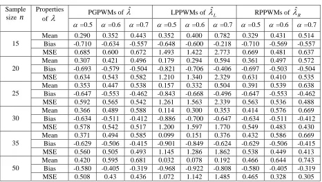
Table 5: Mean, Bias and MSE of PGPWMs Parameter Estimators for EE distribution from Doubly, Left and Right Censoring for u1 0.1 and

4 . 0

2 

u

Sample size n

Properties of 

PGPWMs of ˆ LPPWMs of ˆ_L RPPWMs of ˆ_R

 =0.5 =0.6 =0.7 =0.5  =0.6 =0.7 =0.5 =0.6  =0.7

15

Mean 0.290 0.352 0.443 0.352 0.400 0.782 0.329 0.431 0.514

Bias -0.710 -0.634 -0.557 -0.648 -0.600 -0.218 -0.710 -0.569 -0.557

MSE 0.685 0.600 0.672 1.493 1.422 2.773 0.669 0.481 0.637

20

Mean 0.307 0.421 0.496 0.179 0.294 0.594 0.361 0.497 0.572

Bias -0.693 -0.579 -0.504 -0.821 -0.706 -0.406 -0.697 -0.503 -0.504

MSE 0.634 0.543 0.582 1.210 1.340 2.329 0.631 0.410 0.535

25

Mean 0.353 0.447 0.538 0.157 0.332 0.504 0.391 0.539 0.638

Bias -0.647 -0.553 -0.462 -0.843 -0.668 -0.496 -0.647 -0.553 -0.462

MSE 0.592 0.565 0.542 1.261 1.563 2.339 0.563 0.536 0.488

30

Mean 0.366 0.489 0.588 0.114 0.300 0.353 0.414 0.576 0.669

Bias -0.634 -0.511 -0.412 -0.886 -0.700 -0.647 -0.634 -0.511 -0.412

MSE 0.578 0.542 0.517 1.200 1.597 1.770 0.549 0.483 0.430

35

Mean 0.371 0.494 0.585 0.099 0.151 0.376 0.432 0.586 0.669

Bias -0.629 -0.506 -0.415 -0.901 -0.849 -0.624 -0.629 -0.506 -0.415

MSE 0.560 0.505 0.493 1.145 1.286 1.862 0.538 0.449 0.413

50

Mean 0.420 0.595 0.681 0.032 0.078 0.192 0.466 0.644 0.743

Bias -0.580 -0.405 -0.319 -0.968 -0.922 -0.808 -0.580 -0.405 -0.319

MSE 0.508 0.43 0.436 1.072 1.142 1.485 0.465 0.328 0.305

Table 6: Mean, Bias and MSE of PPWMs Parameter Estimators for EE distribution from Doubly, Left and Right Censoring for u₁ 0 _and

1

2 

u

Sample size n

Properties of 

PGPWMs of ˆ LPPWMs of ˆ_L RPPWMs of ˆ_R

=0.5 =0.6  =0.7 =0.5 =0.6 =0.7  =0.5  =0.6 =0.7

15

Mean 0.286 0.367 0.472 0.343 0.497 0.562 0.328 0.415 0.535

Bias -0.714 -0.633 -0.528 -0.657 -0.503 -0.437 -0.714 -0.633 -0.528

MSE 0.707 0.686 0.662 1.601 1.923 2.219 0.694 0.659 0.644

20

Mean 0.311 0.400 0.502 0.162 0.332 0.442 0.359 0.469 0.561

Bias -0.689 -0.600 -0.498 -0.838 -0.668 -0.558 -0.689 -0.600 -0.498

MSE 0.641 0.606 0.633 1.193 1.653 2.043 0.625 0.593 0.571

25

Mean 0.337 0.454 0.531 0.124 0.243 0.442 0.381 0.505 0.600

Bias -0.663 -0.546 -0.469 -0.876 -0.757 -0.558 -0.663 -0.546 -0.469

MSE 0.596 0.553 0.564 1.201 1.514 2.085 0.583 0.519 0.517

30

Mean 0.350 0.481 0.566 0.070 0.158 0.328 0.409 0.547 0.656

Bias -0.650 -0.519 -0.434 -0.093 -0.842 -0.672 -0.650 -0.519 -0.434

MSE 0.585 0.542 0.556 1.104 1.291 1.796 0.578 0.480 0.489

35

Mean 0.371 0.494 0.600 0.040 0.168 0.326 0.428 0.566 0.685

Bias -0.629 -0.506 -0.400 -0.960 -0.832 -0.674 -0.629 -0.506 -0.400

MSE 0.562 0.515 0.514 1.050 1.345 1.834 0.547 0.468 0.452

50

Mean 0.405 0.519 0.682 0.012 0.077 0.135 0.457 0.637 0.733

Bias -0.595 -0.481 -0.318 -0.988 -0.923 -0.865 -0.595 -0.481 -0.318

Table 7: Mean, Bias and MSE of the shape parameter estimators for EE distribution by the methods of PGPWMs with doubly, left and right censored based on real data

Sample size n

Properties Of 

1

u u₂

28 . 5

 

PGPWMs of ˆ LPGPWMs of ˆ RPGPWMs of ˆ

23

Mean

0.5 1.5

0.8948 1.1401 0.9034

Bias 0.3943 0.6401 0.4034

MSE 0.1554 0.4098 0.1627

Mean

0.1 0.4

0.8308 1.0817 0.9472

Bias 0.3308 0.5817 0.4472

MSE 0.1094 0.3384 0.2000

Mean

0 1

0.9383 1.2248 1.0088

Bias 0.4383 0.7248 0.5088

MSE 0.1921 0.5254 0.2589

Table 8: Mean, Bias and MSE of the scale parameter estimators for EE distribution by the methods of PGPWMs with doubly, left and right censored based on real data

Sample size n

Properties Of 

1

u u₂

1

 

PGPWMs of ˆ LPGPWMs of ˆ RPGPWMs of ˆ

23

Mean

0.5 1.5

0.0320 0.0263 0.0314

Bias -0.9680 -0.9688 -0.9686

MSE 0.9370 0.9386 0.9382

Mean

0.1 0.4

0.1547 0.0279 0.0282

Bias -0.8453 -0.9664 -0.9659

MSE 0.7145 0.9339 0.9300

Mean

0 1

0.0261 0.0098 0.0211

Bias -0.9690 -0.9902 -0.9761