R E S E A R C H
Open Access
A graph modification approach for finding
core–periphery structures in protein
interaction networks
Sharon Bruckner
1, Falk Hüffner
2and Christian Komusiewicz
2*Abstract
The core–periphery model for protein interaction (PPI) networks assumes that protein complexes in these networks consist of a dense core and a possibly sparse periphery that is adjacent to vertices in the core of the complex. In this work, we aim at uncovering a global core–periphery structure for a given PPI network. We propose two exact graph-theoretic formulations for this task, which aim to fit the input network to a hypothetical ground truth network by a minimum number of edge modifications. In one model each cluster has its own periphery, and in the other the periphery is shared. We first analyze both models from a theoretical point of view, showing their NP-hardness. Then, we devise efficient exact and heuristic algorithms for both models and finally perform an evaluation on subnetworks of theS. cerevisiaePPI network.
Keywords: Protein complexes, Graph classes, NP-hard problems
Background
A fundamental task in the analysis of PPI networks is the identification of protein complexes and functional modules. Herein, a basic assumption is that complexes in a PPI network are strongly connected among them-selves and weakly connected to other complexes [1]. This assumption is usually too strict. To obtain a more realistic network model of protein complexes, several approaches incorporate the core–attachment model of protein complexes [2]. In this model, a complex is con-jectured to consist of a stable core plus some attachment proteins, which have only transient interactions with the core. In graph-theoretic terms, the core thus is a dense subnetwork of the PPI network. The attachment (or: periphery) is less dense, but has edges to one or more cores.
Current methods employing this type of modeling are based onseed growing[3-5]. Here, an initial set of promis-ing small subgraphs is chosen as cores. Then, each core is separately greedily expanded by adding vertices to its
*Correspondence: [email protected]
2Institut für Softwaretechnik und Theoretische Informatik, TU Berlin, Ernst-Reuter-Platz 7, 10587 Berlin, Germany
Full list of author information is available at the end of the article
core or its attachment (in each step, a vertex maximizing some specific objective function is chosen). The aim of these approaches was to predict protein complexes [4,5] or to reveal biological features that are correlated with topological properties of core–periphery structures in networks [3]. In this work, we use core–periphery mod-eling in a different context. Instead of searching forlocal core–periphery structures, we attempt to unravel aglobal core–periphery structure in PPI networks.
To this end, we hypothesize that the true network con-sists of several core–periphery structures. We propose two precise models to describe this. In the first model, the core–periphery structures are disjoint. In the second model, the peripheries may interact with different cores, but the cores are disjoint. Then, we fit the input data to each formal model and evaluate the results on several PPI networks.
Our approach. In spirit, our approach is related to the clique-corruption model of the CAST algorithm for gene expression data clustering [6]. In this model, the input is a similarity graph where edges between vertices indicate similarity. The hypothesis is that the objects correspond-ing to the vertices belong to disjoint biological groups of similar objects, the clusters. In the case of gene expres-sion data, these are assumed to be groups of genes with
the same function. Assuming perfect measurements, the similarity graph is a cluster graph.
Definition 1. A graph G is a cluster graph if each con-nected component of G is a clique.
Because of stochastic measurement noise, the input graph is not a cluster graph. The task is to recover the underlying cluster graph from the input graph. Under the assumption that the errors are independent, the most likely cluster graph is one that disagrees with the input graph on a minimum number of edges. Such a graph can be found by applying a minimum number of edge modifications (that is, edge insertions or edge deletions) to the input graph. This paradigm directly leads to the optimization problem CLUSTEREDITING[7-9].
We now apply this approach to our hypothesis that there is a global core–periphery structure in the PPI networks. In both models detailed here, we assume that all proteins of each core interact with each other; this implies that each core is a clique. We also assume that the proteins in the periphery interact only with the cores but not with each other. Hence, the peripheries are independent sets.
In the first model, we assume that ideally the protein interactions give rise to vertex-disjoint core–periphery structures, that is, there are no interactions between different cores and no interactions between cores and peripheries of other cores. Then each connected compo-nent has at most one core which is a clique and at most one periphery which is an independent set. This is precisely the definition of a split graph.
Definition 2.A graph G = (V,E)is a split graph if V can be partitioned into V1and V2such that G[V1]is an independent set and G[V2]is a clique.
We call the vertices in V1 periphery verticesand the vertices inV2core vertices. Note that the partition for a split graph is not always unique. Split graphs have been previously used to model core–periphery structures in social networks [10]. There, however, the assumption is that the network contains exactly one core–periphery structure. We assume that each connected component is a split graph; we call graphs with this propertysplit clus-ter graphs. Our fitting model is described by the following optimization problem.
SPLITCLUSTEREDITING
Input:An undirected graphG=(V,E). Task:TransformGinto a split cluster graph by applying a minimum number of edge modifications.
In our second model, we allow the vertices in the periph-ery to be attached to an arbitrary number of cores, thereby
connecting the cores. In this model, we thus assume that the cores are disjoint cliques and the vertices of the periphery are an independent set. Such graphs are called monopolar[11].
Definition 3.A graph is monopolar if its vertex set can be two-partitioned into V1 and V2 such that G[V1] is an independent set and G[V2]is a cluster graph. The partition(V1,V2)is called monopolar partition.
Again, we call the vertices inV1periphery vertices and the vertices inV2core vertices. Our second fitting model now is the following.
MONOPOL AREDITING
Input:An undirected graphG=(V,E). Task:TransformGinto a monopolar graph by applying a minimum number of edge modifications and output a monopolar partition.
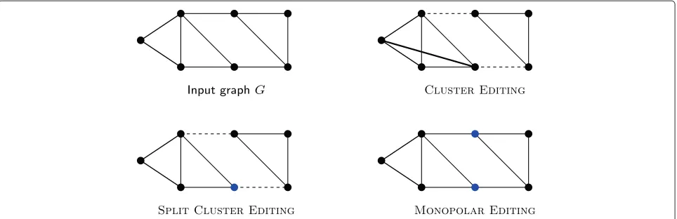
Figure 1 shows an example graph along with optimal solutions for SPLIT CLUSTER EDITING and MONOPO-L AR EDITING and, for comparison, CLUSTER EDITING. Clearly, the models behind SPLITCLUSTEREDITINGand MONOPOL AR EDITING are simplistic and cannot com-pletely reflect biological reality. For example, subunits of protein complexes consisting of two proteins that first interact with each other and subsequently with the core of a protein complex are supported by neither of our models. Nevertheless, our models are less simplistic than pure clustering models that attempt to divide protein interaction networks into disjoint dense clusters. Further-more, there is a clear trade-off between model complexity, algorithmic feasibility of models, and interpretability.
Further related work. In the following, we point to some related work in the literature that is not directly relevant for our algorithms and their evaluation but either consid-ers models of core–periphery structure or optimization problems that are related to SPLITCLUSTEREDITINGor MONOPOL AREDITING.
Della Rossa et al. [12] proposed to compute core– periphery profiles that assign to each vertex a numeri-cal coreness value. The computation of these values is based on a heuristic random-walk model. Their evalua-tion showed that theS. cerevisiaePPI network exhibits a clear core–periphery structure which significantly devi-ates from random networks with the same degree distri-bution. An adaption of the Markov Clustering algorithm MCL that incorporates the core-attachment model for protein complexes was presented by Srihari et al. [13].
Figure 1An example input and optimal solutions to CLUSTEREDITING, SPLITCLUSTEREDITING, and MONOPOLAREDITING. Dashed edges are edge deletions, bold edges are edge insertions. CLUSTEREDITINGand SPLITCLUSTEREDITINGproduce the same two clusters but SPLITCLUSTEREDITING assigns the blue vertex of the size-four cluster to the periphery. In an optimal solution to MONOPOLAREDITINGthe two blue vertices are in the periphery which is shared between two clusters. Note that the number of necessary edge modifications decreases from CLUSTEREDITINGto SPLIT CLUSTEREDITINGto MONOPOLAREDITING.
EDITING is, somewhat surprisingly, solvable in linear time [14]; in fact, the number of required modifications depends only on the degree sequence. Thus, split graphs are recognizable by their degree sequence. Another prob-lem that is related to CLUSTER EDITING is COGRAPH EDITINGwhich asks to destroy inducedP4’s by modifying at most k edges [15]. COGRAPH EDITING has applica-tions in the computation of phylogenies [16]. In a cograph, every connected component has diameter at most two; in split cluster graphs every connected component has diameter at most three.
Finally, a further approach of fitting PPI networks to specific graph classes was proposed by Zotenko et al. [17] who find for a given PPI network a close chordal graph, that is, a graph without induced cycles of length four or more. The modification operation is insertion of edges. One notable difference is that the algorithm may be unable to construct a chordal graph from the input network [17].
Preliminaries. We consider undirected simple graphs G = (V,E)wheren := |V|denotes the number of ver-tices and m := |E| denotes the number of edges. The open neighborhood of a vertex u is defined asN(u) := {v | {u,v} ∈ E}. We denote theneighborhood of a set U byN(U) := u∈UN(u)\U. Thesubgraph induced by a vertex set Sis defined asG[S] :=(S,{{u,v} ∈E|u,v∈S}). One approach to solving NP-hard problems is based on the concept of fixed-parameter tractability [18,19]. Herein, instancesIof a problem come along with a param-eterk, for example the size of a solution. The aim is to obtain a fixed-parameter algorithm, that is, an algorithm with running timef(k)·nO(1)wheref depends only onk.
Such an algorithm is efficient ifkis small andf does not grow too rapidly.
The exponential-time hypothesis (ETH) states that there is a constantc>1 such that 3-SAT cannot be solved in(c−)ntime for any > 0 [20]. Assuming the ETH, tight running time lower bounds can be shown; a sur-vey on ETH-based running time lower bounds is given by Lokshtanov et al. [21]. If it is known that a parameterized problemLdoes not admit a 2o(k)·nO(1)-time algorithm (assuming the ETH), then a polynomial-time reduction from this problem to a problemL with parameterk = O(k)implies thatLcannot be solved in 2o(k)·nO(1)time (assuming the ETH). Note that the parameter in this case may also be the number of vertices or the number of edges of a graph.
Combinatorial properties and complexity
Before presenting concrete algorithmic approaches for the two optimization problems, we show some properties of split cluster graphs and monopolar graphs which will be useful in the various algorithms. Furthermore, we present computational hardness results for the problems which will justify the use of integer linear programming (ILP) and heuristic approaches.
Split cluster editing
Each connected component of the solution has to be a split graph. These graphs can be characterized by forbid-den induced subgraphs (see Figure 2).
Lemma 1([22]).A graph G is a split graph if and only if G does not contain an induced subgraph that is a pair of disjoint edges or a cycle of four or five edges, that is, G is
Figure 2The forbidden induced subgraphs for split graphs (2K2,C4, andC5) and for split cluster graphs (C4,C5,P5, necktie, and bowtie).
To obtain a characterization for split cluster graphs, we need to characterize the existence of 2K2’s within con-nected components. The following lemma will be useful for this purpose.
Lemma 2.If a connected graph contains a 2K2 as induced subgraph, then it contains a2K2 = (V,E)such that there is a vertex v∈/Vthat is adjacent to at least one vertex of each K2of(V,E).
Proof. LetGcontain the 2K2{x1,x2},{y1,y2}as induced subgraph. Without loss of generality, let the shortest path between anyxi,yj beP = (x1 = p1,p2,. . .,pk = y1). Clearly,k > 2. Ifk =3, thenx1andy1are both adjacent top2. Otherwise, ifk=4, then{x2,x1=p1},{p3,p4=y1} is a 2K2andx1andp3are both adjacent top2. Finally, if k > 4, then P contains aP5as induced subgraph. The four outer vertices of thisP5induce a 2K2whoseK2’s each contain a neighbor of the middle vertex.
We can now provide a characterization of split cluster graphs (see Figure 2).
Theorem 1.A graph G is a split cluster graph if and only if G is a(C4,C5,P5,necktie,bowtie)-free graph.
Proof. LetGbe a split cluster graph, that is, every con-nected component is a split graph. Clearly, Gdoes not contain aC4orC5. If a connected component ofG con-tains aP5, then omitting the middle vertex of theP5yields a 2K2, which contradicts the assumption that the con-nected component is a split graph. The same argument shows that the graph cannot contain a necktie or bowtie.
Conversely, let G be (C4,C5,P5, necktie, bowtie)-free. Clearly, no connected component contains a C4 or C5. Assume towards a contradiction that a connected compo-nent contains a 2K2consisting of theK2’s{a,b}and{c,d}. Then according to Lemma 2 there is a vertexvwhich is, without loss of generality, adjacent toaandc. If no other edges between the 2K2andvexist, then{a,b,v,c,d}is a P5. Adding exactly one of{b,v}or{d,v}creates a necktie, and adding both edges results in a bowtie. No other edges are possible, since there are no edges between{a,b}and {c,d}.
This leads to a linear-time algorithm for checking whether a graph is a split cluster graph.
Theorem 2.There is an algorithm that determines in O(n+m)time whether a graph is a split cluster graph and outputs a forbidden induced subgraph if this is not the case.
Proof. For each connected component, we run an algo-rithm by Heggernes and Kratsch [23] that checks in linear time whether a graph is a split graph, and if not, pro-duces a 2K2,C4, orC5. If the forbidden subgraph is aC4 orC5, we are done. If it is a 2K2, then we find, using the method described in the proof of Lemma 2, in linear time an induced 2K2such that there is a vertexvthat is adjacent to at least one vertex in eachK2. The subgraph induced by this 2K2plusvis either aP5, necktie, or bowtie, as shown in the proof of Theorem 1.
In contrast, SPLIT CLUSTER EDITINGis NP-hard even in restricted cases. Before proving the hardness, we make the following observation that follows from a simple local improvement argument. It will be used in our hardness proof and also in our algorithms.
Observation 1.There is an optimal solution to SPLIT CLUSTEREDITINGsuch that
• every degree-one vertex whose neighbor has degree at least two is a periphery vertex, and
• no inserted edge is incident with a periphery vertex.
Theorem 3. SPLITCLUSTEREDITINGis NP-hard even on graphs with maximum degree 10. Further, it cannot be solved in2o(k)·nO(1)or2o(n)·nO(1)time if the exponential-time hypothesis (ETH) is true.
Proof. We reduce from CLUSTEREDITING:
Input:An undirected graphG=(V,E)and an integerk.
CLUSTEREDITINGis NP-hard [24], even if the maxi-mum degree of the input graph is five [25] and it cannot be solved in 2o(k)·nO(1)time assuming ETH [25,26].
The reduction works as follows; we assume that the original instance does not contain isolated vertices. Given an instance (G,k) of CLUSTER EDITING, build a graphG = (V,E)that has the same vertices and edges asGand degG(v)additional degree-one vertices attached to eachv∈V.
We show that G can be transformed by at most k edge modifications into a cluster graph if and only ifG has a split cluster editing set of size at most k. First, if a set S of at most k edge modifications transforms G into a cluster graph G˜, then performing the same modifications on G transforms G into a split cluster graph G˜: Each connected component of G˜ contains a cliqueK ofG˜ plus degG(v)degree-one vertices adjacent to eachv∈ K. The set of these degree-one vertices is an independent set.
For the other direction, we show that there is a minimum-cardinality edge modification setSthat trans-formsGinto a split cluster graphG˜, such that perform-ingSonGtransformsGinto a cluster graph. By Obser-vation 1 and the fact that each vertex in Ghas degree at least one, we can assume that every vertex inV\V is a periphery vertex in G˜. Consider some vertex v ∈ V. If v is a periphery vertex in G˜, then all degG(v) edges between v and V \V are deleted (there are no edges between periphery vertices). Then, however, a solu-tion with the same cost is to delete all degG(v) edges betweenvandV instead. This solution makesva core vertex with neighbors inV only. Hence, we can assume that S makes every vertex in V a core vertex. SinceG˜ is a split cluster graph, each core is a clique and different cores are disjoint. Hence,S transformsGinto a cluster graph.
This shows the correctness of the reduction. The hard-ness results follow from the previous hardhard-ness results and the fact that the solution size remains the same and that the maximum degree of the constructed graphGis exactly twice the maximum degree ofG.
This hardness result motivates the study of algorith-mic approaches such as fixed-parameter algorithms or ILP formulations. For example, SPLITCLUSTEREDITING is fixed-parameter tractable for the parameter number of edge modifications k by the following search tree algo-rithm: Check whether the graph contains a forbidden subgraph. If this is the case, branch into the possibili-ties to destroy this subgraph. In each recursive branch, the number of allowed edge modifications decreases by one. Furthermore, since the largest forbidden subgraph has five vertices, at most ten possibilities for edge inser-tions or deleinser-tions have to be considered to destroy a
forbidden subgraph. By Theorem 2, forbidden subgraphs can be found inO(n+m)time. Altogether, this implies the following.
Theorem 4.SPLIT CLUSTER EDITING can be solved in O(10k·(n+m))time.
This result is purely of theoretical interest. With fur-ther improvements of the search tree algorithm, practical running times might be achievable.
For example, one could focus on improving the base of the exponential factor by a more elaborate case distinc-tion, either designed manually (e. g. [27]) or automatically [28]. Another approach could be to study parameterized data reduction known askernelization[18,19].
Monopolar graphs
The class of monopolar graphs is hereditary, and thus it is characterized by forbidden induced subgraphs. The set of minimal forbidden induced subgraphs, however, is infinite [29]; for example among graphs with five or fewer vertices, only the wheel W4 is forbidden, but there are 11 minimal forbidden subgraphs with six ver-tices. In contrast to the recognition of split cluster graphs, which is possible in linear time by Theorem 2, deciding whether a graph is monopolar is NP-hard [30]. Algorith-mic research is focused on the recognition problem for special graph classes. A fairly general such approach uses a 2-SAT formulation [31,32]. Thus MONOPOL AREDITING is NP-hard already fork=0 edge modifications. As a con-sequence, it is not fixed-parameter tractable with respect to the number of edge modificationskunless P=NP (in contrast to SPLITCLUSTEREDITING).
Solution approaches
To evaluate our model, it is helpful to obtain optimal solu-tions to eliminate or at least estimate the systematic bias that might be introduced by heuristics. We use an integer linear programming (ILP) formulation for this. Since it is not able to solve the hardest instances, we also present a heuristic based on simulated annealing.
Forbidden subgraph ILP
From Theorem 1, we can easily derive an ILP formulation for SPLITCLUSTEREDITING. For each (undirected) pair of vertices{u,v}, we introduce binary variableseuvindicating whether the edge{u,v} is present in the solution graph. Defining¯euv:=1−euv, we have
minimize
{u,v}∈E ¯
euv+
{u,v}∈/E
euvsubject to (1)
{u,v}∈EF ¯
euv+
{u,v}∈/EF
euv≥1∀(VF,EF)∈F,
whereFis the set of forbidden induced subgraphs onV. A constraint of type (2) forces that at least one edge dif-fers from the forbidden subgraph. Since ann-vertex graph may contain(n5) forbidden subgraphs, in practice we use row generation (lazy constraints) and add in a callback only the constraints that are violated; by Theorem 2, we can find a violated constraint in linear time.
The effectivity of ILP solvers is largely based on getting good lower bounds from the LP relaxation. A common technique to improve this further is to addcutting planes, that is, inequalities that are already implied by any inte-gral solution, but that cut off part of the polytope of the LP relaxation. We can derive some cutting planes by strengthening the forbidden subgraph constraints. For a C5, at least two edits are required to obtain a split cluster graph, so we can replace the 1 on the right-hand side by a 2. For aP5uvwxy, we can use
¯
euv+ ¯evw+ ¯ewx+ ¯exy+ 1
2euw+evx+ 1 2ewy+
1 2exu +1
2eyv≥1. (3)
A factor12is permissible for edits that require at least one more edit; for example inserting{u,w}produces a necktie. The summand euy is omitted, since this insertion pro-duces aC5, which needs at least two more edits. Similar strengthenings are possible for neckties and bowties.
Partition variable ILP
Since monopolar graphs have infinitely many forbidden subgraphs, which are NP-hard to find, the forbidden sub-graph ILP formulation is not feasible for MONOPOL AR EDITING. We show an alternative formulation based on the observation that if we correctly guess the partition into core and independent set vertices, we can get a simpler forbidden subgraph characterization for both split cluster graphs and monopolar graphs.
Lemma 3. Let G = (V,E)be a graph and C ˙∪I = V a partition of the vertices. Then G is a split cluster graph with core vertices C and periphery vertices I if and only if G does not contain an edge with both endpoints in I, nor an induced P3with both endpoints in C.
Proof. “⇒”: We show the contraposition. Thus assume that there is an edge with both endpoints in I or an induced P3 with both endpoints inC. Then I is not an independent set or C does not form a clique in each connected component, respectively.
“⇐”: We again show the contraposition. If Gis not a split cluster graph with core verticesCand periphery ver-ticesI, then it must contain an edge with both endpoints in I, or C ∩H does not induce a clique for some con-nected componentH ofG. In the first case we are done;
in the second case, there are two verticesu,v∈ Cin the same connected component with{u,v} ∈/ E. Consider a shortest path(u = p1,. . .,pl = v)fromutov. If it con-tains a periphery vertexpi ∈ I, thenpi−1,pi,pi+1forms a forbidden subgraph. Otherwise,p1,p2,p3is one.
For annotated monopolar graphs, the situation is even simpler. By Definition 3, the two-partition into C andI exactly demands thatIis an independent set andG[C] is a cluster graph or, equivalently,P3-free.
Lemma 4. Let G = (V,E)be a graph and C ˙∪I = V a partition of the vertices. Then G is a monopolar graph with core vertices C and periphery vertices I if and only if it does not contain an edge with both endpoints in I, nor an induced P3whose vertices are contained in C.
Proof. “⇒”: This follows directly from Definition 3. “⇐”: IfG is not monopolar with core vertices C and periphery vertices I, then it must contain an edge with both endpoints inI, orG[C] is not a cluster graph. In the first case we are done; in the second case, there is aP3 with all vertices inC, since that is the forbidden induced subgraph for cluster graphs.
From Lemma 3, we can derive an ILP formulation for SPLITCLUSTEREDITING. As before, we use binary vari-ableseuv indicating whether the edge{u,v}is present in the solution graph. In addition, we introduce binary vari-ablescuindicating whether a vertexuis part of the core. Defininge¯uv := 1−euv and¯cu := 1−cu, and fixing an arbitrary order on the vertices, we have
minimize
{u,v}∈E ¯
euv+
{u,v}∈/E
euvsubject to (4)
cu+cv+ ¯euv≥1∀u,v (5) ¯
euv+ ¯evw+euw+ ¯cu+ ¯cw≥1∀u=v,v=w>u. (6)
Herein, Constraint (5) forces that the periphery vertices are an independent set and Constraint (6) forces that core vertices in the same connected component form a clique. For MONOPOL AREDITING, we replace Constraint (6) by
¯
euv+ ¯evw+euw+ ¯cu+ ¯cv+ ¯cw≥1∀u=v,v=w>u (7)
which forces that the graph induced by the core vertices is a cluster graph.
Data reduction
modifications. Unfortunately, the data reduction rules we devised for SPLITCLUSTEREDITINGwere not applicable to our real-world test instances. However, Observation 1 allows us to fix the values of some variables of Con-straints (4) to (6) in the partition variable ILP for SPLIT CLUSTEREDITING: if a vertexuhas only one vertexvas neighbor and deg(v) > 1, then setcu = 0 andeuw = 0 for allw = v. Since our instances have many degree-one vertices, this considerably reduces the size of the ILPs.
Heuristics
The integer linear programming approach is not able to solve the hardest of our instances. Thus, we employ the well-knownsimulated annealingheuristic. This is a local search method, where we try a random modification of our current solution, and accept it if it improves the objec-tive; but to escape local minima, we also accept it with a small probability if it makes the objective worse. More precisely, a change in the objective ofis accepted with probability exp(−/T), where the factor T is reduced over the course of the algorithm down to zero, such that the algorithm initially explores a larger part of the search space, but eventually settles in a local minimum. We restart the simulated annealing algorithm, where each repetition has a fixed number of steps.
For SPLITCLUSTEREDITING, we start with a clustering where each vertex is a singleton. As random modifica-tion, we move a vertex to a cluster that contains one of its neighbors. Since this allows only a decrease in the num-ber of clusters, we also allow moving a vertex into an empty cluster. For a fixed clustering, the optimal number of modifications can be computed in linear time by count-ing the edges between clusters and computcount-ing for each cluster a solution for SPLITEDITINGin linear time [14]. For MONOPOL AR EDITING, we additionally have a set representing the shared periphery. Accordingly, we allow moving a vertex into another cluster or into the indepen-dent set. Here, the optimal number of modifications for a fixed clustering can also be calculated in linear time: all edges in the independent set are deleted, all edges between clusters are deleted, and all missing edges within clusters are added.
Experimental results
We test exact algorithms and heuristics for SPLIT CLUS-TEREDITING(SCE) and MONOPOL AREDITING(ME) on several PPI networks, and perform a biological evaluation of the modules found. We use three known methods for comparison.
• The algorithm by Luo et al. [3] (“LUO” for short) produces clusters with core and periphery, like SCE, but the clusters may overlap and might not cover the whole graph. LUOproduces two types of
core–periphery structures, those with a dense core, calledk -plex core, and those with a star core. In the comparison, we consider only the structures with k -plex cores, since this model is closer to our models. For periphery, we consider only neighbors of the core (called 1-periphery by Luo et al. [3]) and not vertices with distance two to the core (called 2-periphery). • The SCAN algorithm [35], like ME, partitions the graph vertices into “clusters”, which we interpret as cores, and “hubs” and “outliers”, which we interpret as periphery. SCAN is run with several parameter combinations, obtaining different results. For consistency, we select the results where the clusters have the highest modularity, as reported by the SCAN program itself.
• In addition, we compare the solutions of SCE and ME with optimal solutions of CLUSTEREDITING(CE) (see Section ‘Split cluster editing’ for a formal problem definition). The result of such a solution is a cluster graph and the size-1 clusters of this cluster graph are an independent set. Accordingly, we interpret the size-1 clusters as periphery. We solve CE by a simple ILP with row generation, using the characterization by the forbidden subgraphP3.
Experimental setup
Implementation details. The ILPs and the simulated annealing heuristic were implemented in C++ and com-piled with the GNU g++ 4.7.2 compiler. As ILP solver, we used CPLEX 12.6.0. For both formulations, we use the heuristic solution found after 10 rounds as MIP start. For the forbidden subgraph formulation (Section ‘Forbid- den subgraph ILP’), in a lazy constraint callback, we find a forbidden subgraph using Theorem 2 and add the corresponding inequality of type (2) to the model. We then delete one of its vertices and try to find another forbidden subgraph, adding up to n inequalities per callback.
For the partition variable formulation (Section ‘Partition variable ILP’), we initially add all independent set con-straints (5) and thoseP3constraints ((6), (7)) for which the verticesu,v,winduce aP3in the input graph. In a lazy constraint callback, we add violatedP3constraints (usu-ally only a few are needed). These constraints are also used as cutting planes, that is, we already add them in a cut-ting plane callback when they are violated by the fractional solution. In addition, we use the forbidden subgraphs C4 andP5 for SCE and the forbidden subgraph W4 for ME as cutting planes (Eq. 2). In the cutting plane call-backs, we add the 500 inequalities which are violated the most, if the violation is at least 0.3 (these parameters were heuristically determined).
The test machine is a 4-core 3.6 GHz Intel Xeon E5-1620 (Sandy Bridge-E) with 10 MB L3 cache and 64 GB main memory, running Debian GNU/Linux 7.0. CPLEX was allowed to use up to 8 threads, and we report wall clock times.
Data. For comparison of the algorithms, we first use ran-dom graphs, where each possible edge is present with probabilityp, to examine variability of running times and limits of feasibility. For more realistic data, we generate subnetworks of the S. cerevisiae(yeast) protein interac-tion network from BioGRID [36]. Our networks contain only physical interactions. For each Gene Ontology (GO) term in the annotations of the Saccharomyces Genome Database (SGD) [37], we extract the subnetwork induced by only those proteins that are annotated with this term. We omit networks with fewer than 30 vertices (these can all be solved in less than one second). This yields 178 graphs with up to 2198 vertices, with a median of 66 vertices and 226 edges.
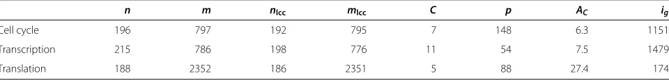
For the biological evaluation, we focus on three partic-ular subnetworks, corresponding to three essential pro-cesses: cell cycle, translation, and transcription.a These are important subnetworks known to contain complexes. Table 1 shows some properties of these networks.
Biological evaluation. We evaluate our results using the following measures. First, we examine the coherence of the GO terms in our modules using the semantic sim-ilarity score calculated by G-SESAME [38]. We use this score to test the hypothesis that the cores are more sta-ble than the peripheries. If the hypothesis is true, then the GO terms within a core should be more similar than the GO terms in the periphery. Hence, the pairwise similarity score within the core should be higher than in the periph-ery. We test only terms relating to process, not function, since proteins in the same complex play a role in the same biological process. Since ME, SCAN, and CE return mul-tiple cores and only a single periphery, we assign to each clusterC its neighborhoodN(C)as periphery. We con-sider only clusters with at least two core vertices and one periphery vertex.
Next, we compare the resulting clusters with known protein complexes from the CYC2008 database [39]. Since
the networks we analyze are subnetworks of the larger yeast network, we discard for each network the CYC2008 complexes that have less than 50% of their vertices in the current subnetwork, restrict them to proteins contained in the current subnetwork, and then discard those with fewer than three proteins. We test the overlap between the algorithm results and these complexes, treating the complexes as the “ground truth”. We expect that the cores mostly correspond to complexes and that the periphery may contain complex vertices plus further vertices.
Results
Random networks
Figure 3 shows running times for random graphs using the fastest ILP version (using partition variables and cutting planes). Each box represents 25 runs. For SCE, running times show large variation (note the logarithmic scale). Densityp = 0.3 here yields harder instances than either denser or sparser instances. Already for n = 22, two instances withp=0.3 could not be solved with available memory, although another one takes only three seconds. For ME andp = 0.1 orp = 0.3, there are fewer outliers and the instances can be solved much quicker than for the SCE model. Running times and variance of running time seem to increase monotonously with density, how-ever. Thus, forp=0.5 SCE could be solved quicker than ME.
The heuristic optimally solves SCE for all instances with known optimal solution; for ME, it is off by one for five instances.
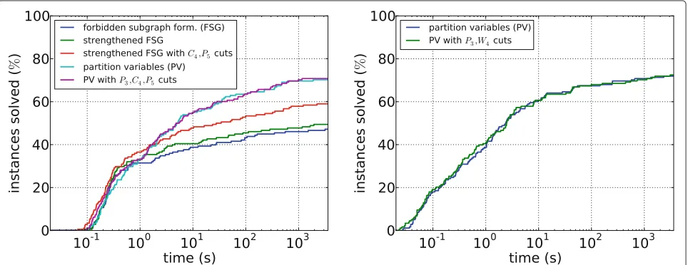
PPI subnetworks
Figure 4 shows running times for the different ILP approaches on PPI subnetworks. Overall, we can observe that these instances are much easier than the random graph instances. For SCE with the forbidden subgraph for-mulation, we see that the strengthened inequalities such as Constraint (3) allow to solve more instances, and that using theP5(in our instances the most frequent forbid-den subgraph) not only as a forbidforbid-den subgraph but also as a cutting plane further improves running time. How-ever, neither version is as effective as the partition variable formulation. Here, using forbidden subgraphs as cutting planes has less effect, solving only one more instance.
Table 1 Input properties of the process networks
n m nlcc mlcc C p AC ig
Cell cycle 196 797 192 795 7 148 6.3 1151
Transcription 215 786 198 776 11 54 7.5 1479
Translation 188 2352 186 2351 5 88 27.4 174
Figure 3Running times for random graphs. Left: SPLITCLUSTEREDITING; right: MONOPOLAREDITING. A star indicates an instance that was aborted due to insufficient memory.
This is probably because adding the initial constraints ((5) to (7)) already produces a fairly tight relaxation. Moreover, finding the cutting planes is quite slow.
For ME, we note that instances can be solved slightly quicker in general, consistent with the observations on sparse random networks. Using W4 (the smallest for-bidden subgraph for monopolar graphs) as a cutting plane also helps little, solving one more instance, but might be useful for difficult instances with long running time.
The heuristic for SCE finds an optimal solution for all 126 instances for which the optimal solution size is known. The ME heuristic optimally solves 104 of 129 instances for which the optimal solution size is known. The average error is very small (0.61), but for one instance the heuristic produces a solution size too high by 27. Possibly the independent set, which interacts with all clusters, makes local search approaches less effective here compared to SCE.
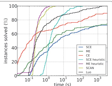
Figure 5 shows the running times for the fastest ILP approaches, that is, the partition variable ILPs with cuts, and the heuristics for both problems. Also shown are the running times of SCAN, LUO, and the ILP for CE. For the majority of the instances, the ILP approaches for SCE and ME are much slower than all other methods including the ILP for CE. SCAN and the ME heuristic are the fastest methods, solving each instance in less than a minute and most instances within a second. The SCE heuristic is sub-stantially slower than the ME heuristic; this behavior is consistent with the observations for the ILP approaches. Finally, LUO is comparable with the SCE heuristic: it is faster than the exact ILP approaches but substantially slower than SCAN and the ME heuristic.
Process networks
Our results are summarized in Table 2 (size statistics and average GO term coherence) and Table 3 (complex detection).
Figure 5Running times of the best ILP formulations, of the two heuristics, and of LUOand SCAN for the PPI subnetworks.
Running times and objective function. For SCE, the ILP approach failed to solve the cell cycle and tran-scription network, and for ME, it failed to solve the transcription network, with CPLEX running out of mem-ory in each case. Thus, consistent with the previous types of instances, the theoretically harder ME problem was easier to solve in practice. This could be explained by the fact that the numberkof necessary modifications is much lower, which could reduce the size of the branch-and-bound tree. For two of the three optimally solved instances, the heuristic finds the optimal solution within one minute. For the third instance (ME transcription) it finds the optimal solution only after several hours; after one minute, it is 2.9% too large. This indicates the heuris-tic gives good results, and in the following, we use the heuristic solution for the three instances not solvable by ILP. From experiments with other networks, we conjec-ture that the heuristic SCE solutions are optimal; we are less sure about the heuristic solutions for ME.
As for the PPI subnetworks, the SCAN algorithm runs very fast, finishing within seconds on all three networks; the LUO algorithm is considerably slower as it needs
several minutes on the translation network. CE is again slower than LUObut still considerably faster than SCE and ME.
Cluster statistics and GO term coherence. Table 2 gives an overview of the number and average sizes of the out-put clusters and of their average GO term coherence in core and periphery. We say that a cluster isnontrivialif it has at least three vertices and at least two core vertices. We describe the results for the cell cycle network in more detail since the results here are the most representative of the three networks. Then, we summarize our findings for the transcription and translation network.
The SCE solution identifies 14 nontrivial clusters; all other clusters are singletons. Only for one of the 14 non-trivial clusters, the GO term coherence is lower in the core than in the periphery (for two clusters the scoring tool does not return a result, four clusters have empty periph-eries). This is in line with the hypothesis that cores have higher GO term coherence than peripheries.
The ME result contains more nontrivial clusters than SCE (24). Compared to SCE, clusters have on average about the same size, but a slightly smaller core and a slightly larger periphery (recall that a periphery vertex may occur in more than one cluster). The average coher-ence in the cores is 0.58, lower than for SCE (0.64), this might be due to the fact that the cores are smaller for ME. On average, coherence in the periphery is much lower than in the cores, but for six clusters it is higher than in the core.
SCAN identifies 7 hubs and 41 outliers, which then comprise the periphery. There are even more nontrivial clusters than for ME. Clusters are smaller than for SCE or ME, in particular the periphery has on average only 4.4 vertices as opposed to 7.3 for SCE or 9.8 for ME. Coher-ence on cores is similar to SCE and ME, and also lower for the periphery.
LUOoutputs only large clusters (this is true for all sub-networks we tested). For the cell cycle network, 16 clusters are identified, each having at least 5 proteins in the cores, and 3 in the periphery, and the largest having 15 proteins in the core and 126 in the periphery (for SCE, one cluster
Table 2 Solution statistics and average GO term coherence for the process networks
Cell-cycle Transcription Translation
k K c¯ p¯ ct cc cp k K c¯ p¯ ct cc cp k K c¯ p¯ ct cc cp
SCE 321 14 5 7 0.60 0.64 0.40 273 14 6 6 0.54 0.56 0.57 308 6 13 14 0.70 0.73 0.69
ME 126 24 3 9 0.45 0.57 0.40 106 26 3 7 0.50 0.60 0.54 240 11 8 12 0.59 0.61 0.54
SCAN — 28 5 4 0.41 0.62 0.34 — 29 4 3 0.48 0.59 0.47 — 5 30 4 0.66 0.66 0.76
Luo — 16 9 63 0.34 0.50 0.31 — 12 8 41 0.40 0.52 0.38 — 4 24 24 0.72 0.84 0.67
CE 461 28 4 1 0.51 0.51 0.38 392 28 4 1 0.56 0.57 0.68 937 10 11 4 0.71 0.73 0.71
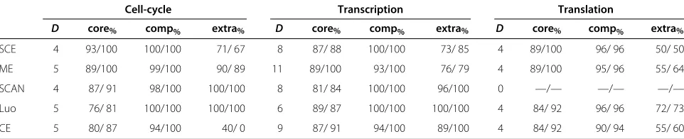
Table 3 Complex detection statistics for the process networks
Cell-cycle Transcription Translation
D core% comp% extra% D core% comp% extra% D core% comp% extra%
SCE 4 93/100 100/100 71/ 67 8 87/ 88 100/100 73/ 85 4 89/100 96/ 96 50/ 50
ME 5 89/100 99/100 90/ 89 11 89/100 93/100 76/ 79 4 89/100 95/ 96 55/ 64
SCAN 4 87/ 91 98/100 100/100 8 81/ 84 100/100 96/100 0 —/— —/— —/—
Luo 5 76/ 81 100/100 100/100 6 89/ 87 100/100 100/100 4 84/ 92 96/ 96 72/ 73
CE 5 80/ 87 94/100 40/ 0 9 87/ 91 94/100 89/100 4 84/ 92 90/ 94 55/ 60
Here,Dis the number of detected complexes, core%is among the detected complexes the mean/median percentage of core vertices that are in this complex, comp%
is the mean/median percentage of complex proteins that are in the cluster, and extra%is the mean/median percentage of periphery proteins that are not in the cluster.
has 10 proteins in the core and 56 in the periphery, and all other clusters for the three other methods have cores of at most 16 and peripheries of at most 30 vertices). The cores have much lower coherence on average than the other methods, but again coherence in the periphery is even lower.
CE outputs many nontrivial clusters, on average the cores and periphery are smaller than for SCE and ME. The average coherence is lower than for SCE and ME, but again the average coherence is higher in the core than in the periphery.
We now describe the results for the transcription net-work. Again, ME outputs the smallest cores, followed by SCAN and CE. LUOagain finds the largest cores and also the largest peripheries. Concerning GO term analysis, we see a similar pattern here that LUOhas worse coherence. The average core coherence is the highest for ME and, unlike CE and SCE, the average coherence is higher in the cores than in the periphery for ME.
In the translation network, ME outputs the most non-trivial clusters, followed by CE and SCE. SCAN and LUO output the fewest nontrivial clusters (5 and 4, respec-tively). LUO has the best coherence values here. The average coherence is higher for CE than for ME but the difference between the average core and periphery coher-ence is less pronounced in CE than in ME.
Complex detection. Table 3 gives an overview of the number of detected complexes. Again, we describe the results for the cell cycle network in more detail and then summarize our findings for the transcription and transla-tion network.
Following our hypothesis, we say that a complex is detected by a cluster if at least 50% of the core belongs to the complex and at least 50% of the complex belongs to the cluster. Out of the seven complexes, three are detected without any error (anaphase-promoting, DASH, and Far3p/Far7p/Far8p/Far9p/Far10p/Far11p complex), and one (Mcm2-7) is detected with an error of two addi-tional proteins in the core that are not in the complex. The periphery contains between one and eight extra proteins
that are not in the complex (which is allowed by our hypothesis).
ME detects the same complexes as SCE, and addition-ally the mitotic checkpoint complex. For the anaphase-promoting complex, it misses one protein; all other com-plexes are detected without error.
SCAN detects almost the same complexes as ME (it misses the Mcm2-7 complex). It also has slightly more errors, for example having three extra protein in the core for the anaphase-promoting complex plus one missing. LUOdetects the same complexes as ME without missing any complex proteins but it also finds more extra vertices in the cores. CE detects the same clusters as ME with a slightly higher number of missed complex proteins and extra core proteins.
In the transcription network, the ME method comes out a clear winner: it detects all 11 complexes and has fewer errors than the other methods. CE detects more com-plexes than SCAN and SCE; LUOdetects only 6 complexes for this network.
In the translation network, SCE, ME, LUO, and CE detect the same four complexes. The SCAN algorithm does not seem to deal well with this network, since it does not detect any complex. LUOfinds only four non-trivial clusters, corresponding to the four complexes also detected by SCE and ME; this might also explain why it has the best coherence values here.
Conclusions
Experiment evaluation
The coherence values for cores and peripheries indicate that a division of clusters into core and periphery makes sense. Under the assumption that cores should be more coherent than peripheries, ME and LUO do best with respect to separating cores from periphery.
are not in the complex. Note that when comparing the number of detected complexes, then SCE is at a disadvan-tage, since it can use each protein as periphery only once, while having large peripheries makes it easier to count a complex as detected. One approach here could be to con-sider clusters of size one as shared periphery (as we did for CE). The graph modification-based methods showed a more consistent behavior across the three test networks than LUO(which performs not so well on the transcrip-tion network) and SCAN (which performs not so well on the translation network).
A further notable difference between the algorithms is that LUOoutputs much larger peripheries for each cluster. Thus, the peripheries of the detected complexes contain many proteins which are not known to be in the complex (by our initial hypothesis, these extra proteins are not nec-essarily errors). The other four methods are much more conservative in this regard.
Outlook
Concerning the theoretical analysis of SPLIT CLUSTER EDITINGthe following questions are open: Is SPLIT CLUS-TER EDITING amenable to parameterized data reduc-tion? That is, does SPLIT CLUSTER EDITING admit a polynomial-time reduction to a polynomial-size problem kernel (see [18] for a definition of problem kernel)? Does SPLITCLUSTEREDITINGadmit a constant-factor approx-imation? It would be also interesting to study the SPLIT CLUSTER DELETION problem in which only edge dele-tions are allowed to transform the input graph into a split cluster graph. This variant is also NP-hard by a reduction that is similar to the one presented for SPLIT CLUSTER EDITING.
For MONOPOL AR EDITING it would be interesting to obtain any tractability results, for example by considering combinations of parameters. A first step here could be to study the problem of recognizing monopolar graphs more closely.
There are many further variants of our models that could possibly yield better biological results or have algo-rithmic advantages. For instance, one could restrict the cores to have a certain minimum size. Also, instead of using split graphs as a core–periphery model, one could resort to dense split graphs [10] in which every periph-ery vertex is adjacent to all core vertices. Finally, one could allow some limited amount of interaction between periphery vertices.
Further evaluation of the biological properties of the computed core–periphery structures seems also worth-while. For example, it would be interesting to examine the peripheries more closely in order to determine whether SPLITCLUSTEREDITINGand MONOPOL AREDITINGare too conservative when determining the periphery of a cluster. Finally, one could explore the biological properties
of those clusters that were identified by SPLIT CLUSTER EDITINGor MONOPOL AREDITINGbut that do not cor-respond to known protein complexes from the CYC2008 database (all output clusters are listed in the Additional file 1: Supplemental material).
Endnote
aTo determine the protein subsets corresponding to
each process, we queried BioMart [40] for all yeast genes annotated with the relevant GO terms: GO:0007049 (cell cycle), GO:0006412 (translation), and GO:0006351 (DNA-templated transcription). Note that this gives somewhat different results than using the SGD GO annotations.
Additional file
Additional file 1: Supplemental material.This file contains the source code of the programs that generate the CPLEX ILPs, our input data (the three process networks), and our output clusters. All files are readable as plain text files.
Competing interests
The authors declare that they have no competing interests.
Authors’ contributions
SB conceived the model and developed it with the other authors. Methods and experiments were jointly developed, and FH did the implementation. All authors read and approved the final manuscript.
Acknowledgments
An extended abstract of this article appeared in the Proceedings of the 14th Workshop on Algorithms in Bioinformatics (WABI ’14), volume 8701 of LNCS, Springer, pages 340–351.
Author details
1International Max Planck Research School for Computational Biology and
Scientific Computing, Ihnestr. 63-73, 14195 Berlin, Germany.2Institut für Softwaretechnik und Theoretische Informatik, TU Berlin, Ernst-Reuter-Platz 7, 10587 Berlin, Germany.
Received: 23 December 2014 Accepted: 31 March 2015
References
1. Spirin V, Mirny LA. Protein complexes and functional modules in molecular networks. PNAS. 2003;100(21):12123–8.
2. Gavin A-C, Aloy P, Grandi P, Krause R, Boesche M, Marzioch M, et al. Proteome survey reveals modularity of the yeast cell machinery. Nature. 2006;440(7084):631–6.
3. Luo F, Li B, Wan X-F, Scheuermann R. Core and periphery structures in protein interaction networks. BMC Bioinformatics. 2009;10(Suppl 4):8. 4. Leung HC, Xiang Q, Yiu S-M, Chin FY. Predicting protein complexes from
PPI data: a core-attachment approach. J Comput Biol. 2009;16(2):133–44. 5. Wu M, Li X, Kwoh C-K, Ng S-K. A core-attachment based method to
detect protein complexes in PPI networks. BMC Bioinformatics. 2009;10(1):169.
6. Ben-Dor A, Shamir R, Yakhini Z. Clustering gene expression patterns. J Comput Biol. 1999;6(3-4):281–97.
7. Shamir R, Sharan R, Tsur D. Cluster graph modification problems. Discrete Appl Math. 2004;144(1–2):173–82.
9. Böcker S, Baumbach J. Cluster editing. In: Proceedings of the 9th conference on computability in Europe (CiE ’13). LNCS. Berlin, Heidelberg: Springer; 2013. p. 33–44.
10. Borgatti SP, Everett MG. Models of core/periphery structures. Soc Netw. 1999;21(4):375–95.
11. Chernyak ZA, Chernyak AA. About recognizing(α,β)classes of polar graphs. Discrete Math. 1986;62(2):133–8.
12. Della Rossa F, Dercole F, Piccardi C. Profiling core-periphery network structure by random walkers. Sci Rep. 2013. Article no. 3.
13. Srihari S, Ning K, Leong H. MCL-CAw: a refinement of MCL for detecting yeast complexes from weighted PPI networks by incorporating core-attachment structure. BMC Bioinformatics. 2010;11:504. 14. Hammer PL, Simeone B. The splittance of a graph. Combinatorica.
1981;1(3):275–84.
15. Liu Y, Wang J, Guo J, Chen J. Complexity and parameterized algorithms for cograph editing. Theor Comput Sci. 2012;461:45–54.
16. Hellmuth M, Wieseke N, Lechner M, Lenhof H-P, Middendorf M, Stadler PF. Phylogenomics with paralogs. PNAS. 2015;112(7):2058–63.
17. Zotenko E, Guimarães KS, Jothi R, Przytycka TM. Decomposition of overlapping protein complexes: a graph theoretical method for analyzing static and dynamic protein associations. Algorithms Mol Biol. 2006;1(7):. 18. Downey RG, Fellows MR. Fundamentals of Parameterized Complexity.
Texts in Computer Sci. Berlin, Heidelberg: Springer; 2013.
19. Niedermeier R. Invitation to fixed-parameter algorithms. Oxford: Oxford University Press; 2006.
20. Impagliazzo R, Paturi R, Zane F. Which problems have strongly exponential complexity? J Comput Syst Sci. 2001;63(4):512–30. 21. Lokshtanov D, Marx D, Saurabh S. Lower bounds based on the
exponential time hypothesis. Bull EATCS. 2011;105:41–72. 22. Foldes S, Hammer PL. Split graphs. Congressus Numerantium.
1977;19:311–5.
23. Heggernes P, Kratsch D. Linear-time certifying recognition algorithms and forbidden induced subgraphs. Nord J Comput. 2007;14(1–2):87–108. 24. Kˇrivánek M, Morávek J. NP-hard problems in hierarchical-tree clustering.
Acta Informatica. 1986;23(3):311–23.
25. Fomin FV, Kratsch S, Pilipczuk M, Pilipczuk M, Villanger Y. Subexponential fixed-parameter tractability of cluster editing. CoRR. 2011abs/1112.4419. 26. Komusiewicz C, Uhlmann J. Cluster editing with locally bounded
modifications. Discrete Appl Math. 2012;160(15):2259–70. 27. Liu Y, Wang J, Xu C, Guo J, Chen J. An effective branching strategy
based on structural relationship among multiple forbidden induced subgraphs. J Comb Optimization. 2015;29(1):257–75.
28. Gramm J, Guo J, Hüffner F, Niedermeier R. Automated generation of search tree algorithms for hard graph modification problems. Algorithmica. 2004;39(4):321–47.
29. Berger AJ. Minimal forbidden subgraphs of reducible graph properties. Discussiones Mathematicae Graph Theory. 2001;21(1):111–7. 30. Farrugia A. Vertex-partitioning into fixed additive induced-hereditary
properties is NP-hard. Electron J Combinatorics. 2004;11(1):46. 31. Le VB, Nevries R. Complexity and algorithms for recognizing polar and
monopolar graphs. Theor Comput Sci. 2014;528:1–11. 32. Churchley R, Huang J. Solving partition problems with
colour-bipartitions. Graphs Combinatorics. 2014;30(2):353–64. 33. Cao Y, Chen J. Cluster editing: Kernelization based on edge cuts.
Algorithmica. 2012;64(1):152–69.
34. Chen J, Meng J. A 2kkernel for the cluster editing problem. J Comput Syst Sci. 2012;78(1):211–20.
35. Xu X, Yuruk N, Feng Z, Schweiger TAJ. SCAN: a structural clustering algorithm for networks. In: Proceedings of the 13th ACM SIGKDD international conference on Knowledge Discovery and Data mining (KDD ‘07). New York: ACM; 2007. p. 824–33.
36. Chatr-aryamontri A, Breitkreutz B-J, Heinicke S, Boucher L, Winter AG, Stark C, et al. The BioGRID interaction database: 2013 update. Nucleic Acids Res. 2013;41(D1):816–23.
37. Cherry JM, Hong EL, Amundsen C, Balakrishnan R, Binkley G, Chan ET, et al. Saccharomyces genome database: the genomics resource of budding yeast. Nucleic Acids Res. 2012;40(Database issue):700–5.
38. Du Z, Li L, Chen C-F, Yu PS, Wang JZ. G-SESAME: web tools for GO-term-based gene similarity analysis and knowledge discovery. Nucleic Acids Res. 2009;37(suppl. 2):345–9.
39. Pu S, Wong J, Turner B, Cho E, Wodak SJ. Up-to-date catalogues of yeast protein complexes. Nucleic Acids Res. 2009;37(3):825–31.
40. Kasprzyk A. BioMart: driving a paradigm change in biological data management. Database. 2011;2011.
Submit your next manuscript to BioMed Central and take full advantage of:
• Convenient online submission
• Thorough peer review
• No space constraints or color figure charges
• Immediate publication on acceptance
• Inclusion in PubMed, CAS, Scopus and Google Scholar
• Research which is freely available for redistribution