RESEARCH
A hybrid parameter estimation
algorithm for beta mixtures and applications
to methylation state classification
Christopher Schröder and Sven Rahmann
*Abstract
Background: Mixtures of beta distributions are a flexible tool for modeling data with values on the unit interval, such as methylation levels. However, maximum likelihood parameter estimation with beta distributions suffers from prob-lems because of singularities in the log-likelihood function if some observations take the values 0 or 1.
Methods: While ad-hoc corrections have been proposed to mitigate this problem, we propose a different approach to parameter estimation for beta mixtures where such problems do not arise in the first place. Our algorithm com-bines latent variables with the method of moments instead of maximum likelihood, which has computational advan-tages over the popular EM algorithm.
Results: As an application, we demonstrate that methylation state classification is more accurate when using adap-tive thresholds from beta mixtures than non-adapadap-tive thresholds on observed methylation levels. We also demon-strate that we can accurately infer the number of mixture components.
Conclusions: The hybrid algorithm between likelihood-based component un-mixing and moment-based param-eter estimation is a robust and efficient method for beta mixture estimation. We provide an implementation of the method (“betamix”) as open source software under the MIT license.
Keywords: Mixture model, Beta distribution, Maximum likelihood, Method of moments, EM algorithm, Differential methylation, Classification
© The Author(s) 2017. This article is distributed under the terms of the Creative Commons Attribution 4.0 International License (http://creativecommons.org/licenses/by/4.0/), which permits unrestricted use, distribution, and reproduction in any medium, provided you give appropriate credit to the original author(s) and the source, provide a link to the Creative Commons license, and indicate if changes were made. The Creative Commons Public Domain Dedication waiver (http://creativecommons.org/ publicdomain/zero/1.0/) applies to the data made available in this article, unless otherwise stated.
Background
The beta distribution is a continuous probability distri-bution that takes values in the unit interval [0, 1]. It has been used in several bioinformatics applications [1] to model data that naturally takes values between 0 and 1, such as relative frequencies, probabilities, absolute cor-relation coefficients, or DNA methylation levels of CpG dinucleotides or longer genomic regions. One of the most prominent applications is the estimation of false discov-ery rates (FDRs) from p-value distributions after multiple tests by fitting a beta-uniform mixture (BUM, [2]). By lin-ear scaling, beta distributions can be used to model any quantity that takes values in a finite interval [L,U] ⊂R.
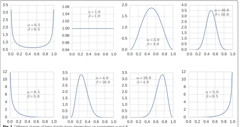
The beta distribution has two parameters α >0 and
β >0 and can take a variety of shapes depending on
whether 0< α <1 or α=1 or α >1 and 0< β <1 or
β=1 or β >1; see Fig. 1. The beta probability density on [0, 1] is
and Ŵ refers to the gamma function
Ŵ(z)=∞
0 xz−1e−xdx with Ŵ(n)=(n−1)! for positive integers n. It can be verified that 1
0 bα,β(x)dx=1. For α=β=1, we obtain the uniform distribution. Section “Preliminaries: Beta distributions” has more details.
(1)
bα,β(x)= 1 B(α,β)·x
α−1·(1−x)β−1,
whereB(α,β)= Ŵ(α)Ŵ(β)
Ŵ(α+β) ,
Open Access
*Correspondence: [email protected]
While a single beta distribution can take a variety of shapes, mixtures of beta distributions are even more flex-ible. Such a mixture has the general form
where c is the number of components, the πj are called mixture coefficients satisfying
j πj=1 and πj≥0, and
the αj,βj are called component parameters. Together, we refer to all of these as model parameters and abbreviate them as θ. The number of components c is often assumed to be a given constant and not part of the parameters to be estimated.
The parameter estimation problem consists of esti-mating θ from n usually independent observed samples (x1,. . .,xn) such that the observations are well explained by the resulting distribution.
Maximum likelihood (ML) estimation (MLE) is a fre-quently used paradigm, consisting of the following opti-mization problem.
(2)
fθ(x)= c
j=1
πj·bαj,βj(x),
(3)
Given(x1,. . .,xn), maximizeL(θ ):= n
i=1 fθ(xi),
or equivalently,L(θ ):= n
i=1
lnfθ(xi).
As we show below in “Preliminaries: Maximum likeli-hood estimation for Beta distributions”, MLE has sig-nificant disadvantages for beta distributions. The main problem is that the likelihood function is not finite (for almost all parameter values) if any of the observed data-points are xi=0 or xi=1.
For mixture distributions, MLE frequently results in a non-concave problem with many local maxima, and one uses heuristics that return a local optimum from given starting parameters. A popular and successful method for parameter optimization in mixtures is the expectation maximization (EM) algorithm [3] that iteratively solves an (easier) ML problem on each estimated component and then re-estimates which datapoints belong to which component. We review the basic EM algorithm below in the Section “Preliminaries: The EM algorithm for beta mixture distributions”.
Because already MLE for a single beta distribution is problematic, EM does not work for beta mixtures, unless ad-hoc corrections are made. We therefore propose a new algorithm for parameter estimation in beta mixtures that we call iterated method of moments. The method is presented in below in the Section “The iterated method of moments”.
states”. Our evaluation therefore focuses on the benefits of beta mixture modeling and parameter estimation using our algorithm for methylation state classification from simulated methylation level data.
Preliminaries Beta distributions
The beta distribution with parameters α >0 and β >0 is
a continuous probability distribution on the unit interval [0, 1] whose density is given by Eq. (1).
If X is a random variable with a beta distribution, then its expected value µ and variance σ2 are
where φ =α+β is often called a precision parameter; large values indicate that the distribution is concentrated. Conversely, the parameters α and β may be expressed in terms of µ and σ2: First, compute
The textbook by Karl Bury [4] has more details about moments and other properties of beta distributions and other distributions used in engineering.
Maximum likelihood estimation for Beta distributions The estimation of parameters in a parameterized distri-bution from n independent samples usually follows the maximum likelihood (ML) paradigm. If θ represents the parameters and fθ(x) is the probability density of a single observation, the goal is to find θ∗ that maximizes L(θ ) as defined in Eq. (3).
Writing γ (y):=lnŴ(y), the beta log-likelihood is
The optimality conditions dL/dα=0 and dL/dβ=0 must be solved numerically and iteratively because the parameters appear in the logarithm of the gamma func-tion. In comparison to a mixture of Gaussians where analytical formulas exist for the ML estimators, this is inconvenient, but the main problem is a different one. The log-likelihood function is not well defined for α�=1 if any of the observations are xi=0, or for β�=1 if any xi=1. Indeed, several implementations of ML estimators for beta distributions (e.g. the R package betareg, see below) throw errors then.
(4)
µ:=E[X] = α
α+β,
σ2:=Var[X] = µ(1−µ)
α+β+1 =
µ(1−µ) 1+φ ,
(5)
φ = µ(1−µ)
σ2 −1; then α=µφ, β=(1−µ)φ.
(6)
L(α,β)=n(γ (α+β)−γ (α)−γ (β))+(α−1)
·
i
lnxi+(β−1)·
i
ln(1−xi).
Note that, in theory, there is no problem, because x∈ {0, 1} is an event of probability zero if the data are truly generated by a beta distribution. Real data, however, in particular observed methylation levels, may very well take these values. This article’s main motivation is the desire to work with observations of x=0 and x=1 in a principled way.
The above problem with MLE for beta distributions has been noted previously, but, to our knowledge, not explic-itly attacked. We here discuss the work-arounds of which we are aware.
Reducing the interval
A typical ad-hoc solution is to linearly rescale the unit interval [0, 1] to a smaller sub-interval [ε, 1−ε] for some small ε >0 or to simply replace values < ε by ε and val-ues >1−ε by 1−ε, such that, in both cases, the result-ing adjusted observations are in [ε, 1−ε].
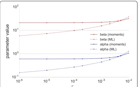
A simple example, which has to our knowledge not been presented before, will show that the resulting parameter estimates depend strongly on the choice of ε in the ML paradigm. Consider 20 observations, 10 of them at x=0, the remaining ten at x=0.01,. . ., 0.10. For dif-ferent values of 0< ε <0.01, replace the ten zeros by ε and compute the ML estimates of α and β. We used the R
package betareg1 [5], which performs numerical ML estimation of logit(µ) and ln(φ), where
logit(µ)=ln(µ/(1−µ)). We then used Eq. (5) to com-pute ML estimates of α and β. We additionally used our
iterated method of moments approach (presented in the remainder of this article) with the same varying ε. In con-trast to MLE, our approach also works with ε=0. The
resulting estimates for α and β are shown in Fig. 2: not only is our approach able to directly use ε=0; it is also
insensitive to the choice of ε for small ε >0.
Using a different objective function
MLE is not the only way to parameter estimation. A more robust way for beta distributions may be to consider the cumulative distribution function (cdf) Fθ(x):=
x
0 fθ(y)dy and compare it with the empirical distribution function F(x)ˆ , the fraction of observations ≤x. One can then choose the parameters θ such that a given distance measure between these functions, such as the Kolmogorov–Smirnov distance
is minimized. This optimization has to be per-formed numerically. We are not aware of specific
1 https://cran.r-project.org/web/packages/betareg/betareg.pdf.
(7)
dKS(Fθ,F)ˆ :=max
implementations of this method for beta distributions or beta mixtures. In this work, we opted for a more direct approach based on the density function.
Using explicit finite‑sample models
As we stated above, in theory, observations of X=0 or X=1 happen with probability zero if X has a continu-ous beta distribution. These observations do happen in reality because either the beta assumption is wrong, or we neglected the fact that the observation comes from a finite-precision observation. For methylation level data, the following model may be a more accurate rep-resentation of the data: To obtain a given datapoint xi, first choose the true methylation level pi from the beta distribution with parameters α,β. Then choose the observation xi from the binomial distribution with suc-cess probability pi and sample size ni. The parameter ni controls the granularity of the observation, and it may be different for each i. In our application setting, pi would be the true methylation level of a specific CpG dinucleo-tide in individual i, and xi would be the observed meth-ylation level with sequencing coverage ni. This richer model captures the relationships between parameters and observations much better, but the estimation pro-cess also becomes more complex, especially if the ni are not available.
Summary
While MLE is known to be statistically efficient for cor-rect data, its results may be sensitive to perturbations of the data. For modeling with beta distributions in par-ticular, the problems of MLE are severe: The likelihood function is not well defined for reasonable datasets that occur in practice, and the solution depends strongly on
ad-hoc parameters introduced to rectify the first prob-lem. Alternative models turn out to be computationally more expensive. Before we can introduce our solution to these problems, we first discuss parameter estimation in mixture models.
The EM algorithm for beta mixture distributions
For parameters θ of mixture models, including each com-ponent’s parameters and the mixture coefficients, the log-likelihood function L(θ )=n
i=1lnfθ(xi), with fθ(xi) as in Eq. (2), frequently has many local maxima; and a globally optimal solution is difficult to compute.
The EM algorithm [3] is a general iterative method for ML parameter estimation with incomplete data. In mixture models, the “missing” data is the information which sample belongs to which component. However, this information can be estimated (given initial param-eter estimates) in the E-step (expectation step) and then used to derive better parameter estimates by ML for each component separately in the M-step (maximization step). Generally, EM converges to a local optimum of the log-likelihood function [6].
E‑step
To estimate the expected responsibility Wi,j of each com-ponent j for each data point xi, the component’s rela-tive probability at that data point is computed, such that
j Wi,j=1 for all i. Averaged responsibility weights yield new mixture coefficients πj+.
M‑step
Using the responsibility weights Wi,j, the components are unmixed, and a separate (weighted) sample is obtained for each component, so their parameters can be esti-mated independently by MLE. The new mixture coeffi-cients’ ML estimates πj+ in Eq. (8) are indeed the averages of the responsibility weights over all samples.
Initialization and termination
EM requires initial parameters before starting with an E-step. The resulting local optimum depends on these initial parameters. It is therefore common to choose the initial parameters either based on additional information (e.g., one component with small values, one with large values), or to re-start EM with different random initiali-zations. Convergence is detected by monitoring relative changes among the log-likelihood or among parameters between iterations and stopping when these changes are below a given tolerance.
(8)
Wi,j =
πjbαj,βj(xi)
k πkbαk,βk(xi)
and πj+= 1
n n
i=1 Wi,j. Fig. 2 Estimated parameter values α (blue) and β (red) from a dataset
Properties and problems with beta mixtures
One of the main reasons why the EM algorithm is pre-dominantly used in practice for mixture estimation is the availability of an objective function (the log-likelihood). By Jensen’s inequality, it increases in each EM iteration, and when it stops increasing, a stationary point has been reached [6]. Locally optimal solutions obtained by two runs with different initializations can be objectively and globally compared by comparing their log-likelihood values.
In beta mixtures, there are several problems with the EM algorithm. First, the responsibility weights Wi,j are not well defined for xi=0 or xi =1 because of the sin-gularities in the likelihood function, as described above. Second, the M-step cannot be carried out if the data contains any such point for the same reason. Third, even if all xi∈ ]0, 1[, the resulting mixtures are sensitive to perturbations of the data. Fourth, because each M-step already involves a numerical iterative maximization, the computational burden over several EM iterations is sig-nificant. We now propose a computationally lightweight algorithm for parameter estimation in beta mixtures that does not suffer from these drawbacks.
The iterated method of moments
With the necessary preliminaries in place, the main idea behind our algorithm can be stated briefly before we dis-cuss the details.
From initial parameters, we proceed iteratively as in the EM framework and alternate between an E-step, which is a small modification of EM’s E-step, and a parameter estimation step, which is not based on the ML paradigm but on Pearson’s method of moments until a stationary point is reached [7].
To estimate Q free parameters, the method of moments’ approach is to choose Q moments of the distri-bution, express them through the parameters and equate them to the corresponding Q sample moments. This usu-ally amounts to solving a system of Q non-linear equa-tions. In simple cases, e.g., for expectation and variance of a single Gaussian distribution, the resulting estimates agree with the ML estimates. Generally, this need not be the case.
The method of moments has been applied directly to mixture distributions. For example, a mixture of two one-dimensional Gaussians has Q=5 parameters: two means µ1,µ2, two variances σ12,σ22 and the weight π1 of the first component. Thus one needs to choose five moments, say mk :=E[Xk] for k=1,. . ., 5 and solve the correspond-ing relationships. Solvcorrespond-ing these equations for many com-ponents (or in high dimensions) seems daunting, even numerically. Also it is not clear whether there is always a unique solution.
For a single beta distribution, however, α and β are
eas-ily estimated from sample mean and variance by Eq. (5), using sample moments instead of true values. Thus, to avoid the problems of MLE in beta distributions, we replace the likelihood maximization step (M-step) in EM by a method of moments estimation step (MM-step) using expectation and variance.
We thus combine the idea of using latent responsibil-ity weights from EM with moment-based estimation, but avoid the problems of pure moment-based estimation (large non-linear equation systems). It may seem surpris-ing that nobody appears to have done this before, but one reason may be the lack of an objective function, as we discuss further below.
Initialization
A general reasonable strategy for beta mixtures is to let each component focus on a certain sub-interval of the unit interval. With c components, we start with one component responsible for values around k/(c−1) for each k=0,. . .,c−1. The expectation and variance of the component near k/(c−1) is initially estimated from the corresponding sample moments of all data points in the interval [(k−1)/(c−1),(k+1)/(c−1)] ∩ [0, 1]. (If an interval contains no data, the component is removed from the model.) Initial mixture coefficients are esti-mated proportionally to the number of data points in that interval.
A second common strategy are randomized start parameters. Instead of using purely uniform random choices, more advanced methods are available, e.g. the D2 -weighted initialization used by k-means++ [8]. We here adapted this idea. Let X⊂ [0, 1] be the set of different data values. Let Y ⊂X be the set of chosen component centers, initially Y = {}. Let DY(x):=miny∈Y |x−y| be the shortest distance of x to any already chosen data point. The initialization then consists of the following steps.
1. Choose the first point y uniformly at random from X; set Y := {y}.
2. Repeat until |Y| =c: Choose y∈X\Y with
prob-ability proportional to DY(y)2; then set Y :=Y ∪ {y}.
3. Sort Y such that y1<· · ·<yc.
4. Expectation and variance of component j=1,. . .,c are initially estimated from the corresponding sample moments of all data points in the interval [yj−0.5, yj+0.5].
E‑step
The E-step is essentially the same as for EM, except that we assign weights explicitly to data points xi =0 and xi =1.
Let j0 be the component index j with the smallest αj. If
there is more than one, choose the one with the largest βj . The j0 component takes full responsibility for all i with
xi =0, i.e., Wi,j0 =1 and Wi,j=0 for j�=j0. Similarly, let j1 be the component index j with the smallest βj (among
several ones, the one with the largest αj). For all i with xi =1, set Wi,j1 =1 and Wi,j =0 for j�=j1.
MM‑step
The MM-step estimates mean and variance of each com-ponent j by responsibility-weighted sample moments,
Then αj and βj are computed according to Eq. (5) and new
mixture coefficients according to Eq. (8).
Termination
Let θq be any real-valued parameter to be estimated and Tq a given threshold for θq. After each MM-step, we com-pare θq (old value) and θq+ (updated value) by the relative change κq:= |θq+−θq|/max
|θ+
q|,|θq|
. (If θq+=θq=0 , we set κq:=0.) We say that θq is stationary if κq<Tq . The algorithm terminates when all parameters are stationary.
Properties
The proposed hybrid method does not have a natural objective function that can be maximized. Therefore we cannot make statements about improvement of such a function, nor can we directly compare two solutions from different initializations by objective function values. It also makes no sense to talk about “local optima”, but, similar to the EM algorithm, there may be several sta-tionary points. We have not yet established whether the method always converges. On the other hand, we have the following desirable property.
Lemma 1 In each MM-step, before updating the com-ponent weights, the expectation of the estimated density equals the sample mean. In particular, this is true at a stationary point.
Proof For a density f we write E[f] for its expectation
x·f(x)dx. For the mixture den-sity (2), we have by linearity of expectation that
(9)
µj= n
i=1Wij·xi n
i=1Wij =
n
i=1 Wij·xi
n·πj
,
σj2= n
i=1Wij·(xi−µj)2
n·πj
.
E[fθ] =
j πjE[bαj,βj] =
j πjµj. Using (9) for µj , this is equal to 1
n
j
i Wijxi = 1ni xi, because
j Wij=1 for each j. Thus E[fθ] equals the sample
mean.
Different objective functions may be substituted for the log-likelihood to compare different stationary points, such as the previously mentioned Kolmogorov–Smirnov distance dKS from Eq. (7). While we do not use it for opti-mization directly (our approach is more lightweight), we can use it to evaluate different stationary points and to estimate the number of necesssary components to repre-sent the data.
Estimating the number of components
The method described so far works for a given and fixed number of components, similarly to the EM algorithm. When the true number of components is unknown, the algorithm has to estimate this number by comparing goodness of fit between the estimated beta mixture and the given data, taking into account the model complex-ity (number of parameters). Usually the Akaike informa-tion criterion (AIC) [9] or Bayesian information criterion (BIC) [10] are minimized for this purpose,
where L∗ is the maximized log-likelihood value, k is the number of free model parameters and n is the sample size. Both criteria favor a good fit but penalize many parameters (complex models with many components). Since our approach is not based on likelihoods, we can-not apply these criteria.
Instead, we use the Kolmogorov–Smirnov distance dKS from Eq. (7) to measure the fit between the estimated mixture cumulative distribution function (cdf), evaluated numerically at each data point, and the empirical cumu-lative distribution function from the data. Naturally, dKS is a decreasing function of the number of components. We fit models with an increasing number of components and stop once dKS drops below a given threshold. Note that for fixed sample size n, the distance dKS can be con-verted into a p-value of the Kolmogorov–Smirnov test and vice versa [11].
Application: classification of methylation states Motivation
We are interested in explaining differences in methyla-tion levels of genomic regions between individuals by genetic variation and would like to find single nucleotide variants (SNVs) whose state correlates well with ylation state. In a diploid genome, we expect the meth-ylation level of a homogeneously methylated region in
(10)
a homogeneous collection of cells to be (close to) 0, 0.5 or 1, and the state of the corresponding region may be called unmethylated, semi-methylated or fully methyl-ated, respectively.
When we measure the methylation level of each CpG dinucleotide in the genome, for example by whole genome bisulfite sequencing (WGBS) [12], we observe fractions M/(M+U) from numbers M and U of reads that indicate methylated and unmethylated cytosines, respectively, at each CpG dinucleotide. These observed fractions differ from the true methylation levels for sev-eral reasons: incomplete bisulfite conversion, sequencing errors, read mapping errors, sampling variance due to a finite number of reads, an inhomogeneous collection of cells being sequenced, the region being heterogeneously methylated, and others.
Therefore we model the observed methylation level by a probability distribution depending on the methylation state. The overall distribution of the observations is cap-tured by a three-component beta mixture model with one component representing values close to zero (unmethyl-ated), one component close to 1/2 (semi-methyl(unmethyl-ated), and one component close to 1 (fully methylated).
Thus the problem is as follows. After seeing n observed methylation levels (x1,. . .,xn), find the originating meth-ylation state for each xi. This is frequently done using rea-sonable fixed cut-off values (that do not depend on the data), e.g. calling values below 0.25 unmethylated, values between 0.25 and 0.75 semi-methylated and values above 0.75 fully methylated [13]. One may leave xi unassigned if the value is too close to one of the cut-off values.
An interesting question is whether choosing thresh-olds adaptively based on the observed sample is advan-tageous in some sense. Depending on the components’ parameters, the value range of the components may over-lap, and perfect separation may not be possible based on the value of xi. Good strategies should be based on the component weights Wij, assigning component j∗(i):= argmaxj Wij to xi. We may refuse to make an assign-ment if there is no clearly dominating component, e.g., if Wi∗:=maxj Wij<T, or if Wi∗−W
(2)
i <T for a given threshold T, where Wi(2) is the second largest weight among the Wij.
Simulation and fitting for class assignment
We investigate the advantages of beta mixture modeling by simulation. In the following, let U be a uniform ran-dom number from [0, 1].
We generate two datasets, each consisting of 1000 three-component mixtures. In the first (second) dataset, we generate 200 (1000) samples per mixture.
To generate a mixture model, we first pick mixture coefficients π =(π1,π2,π3) by drawing U1,U2,U3,
computing s:=
j Uj and setting πj:=Uj/s. This does not generate a uniform element of the probability sim-plex, but induces a bias towards distributions where all components have similar coefficients, which is reason-able for the intended application. The first component represents the unmethylated state; therefore we choose an α≤1 and a β >1 by drawing U1,U2 and setting α:=U1 and β :=1/U2. The third component represents the fully methylated state and is generated symmetrically to the first one. The second component represents the semi-methylated state (0.5) and should have large enough approximately equal α and β. We draw U1,U2 and define γ :=5/min{U1,U2}. We draw V uniformly between 0.9 and 1.1 and set α:=γV and β :=γ /V.
To draw a single random sample x from a mixture dis-tribution, we first draw the component j according to π and then value x from the beta distribution with param-eters αj,βj. After drawing n=200 (dataset 1) or n=1000
(dataset 2) samples, we modify the result as follows. For each mixture sample from dataset 1, we set the three smallest values to 0.0 and the three largest values to 1.0. In dataset 2, we proceed similarly with the 10 smallest and largest values.
We use the algorithm as described above to fit a three component mixture model, with a slightly different ini-tialization. The first component is estimated from the samples in [0, 0.25], the second one from the samples in [0.25, 0.75] and the third one from the samples in [0.75, 1]. The first (last) component is enforced to be fall-ing (risfall-ing) by settfall-ing α1=0.8 (β3=0.8) if it is initially estimated larger.
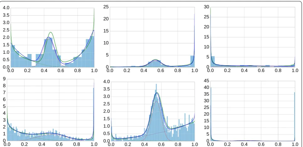
Figure 3 shows examples of generated mixture mod-els, sampled data and fitted models. The examples have been chosen to convey a representative impression of the variety of generated models, from well separated components to close-to-uniform distributions in which the components are difficult to separate. Overall, fitting works well (better for n=1000 than for n=200), but our formal evaluation concerns whether we can infer the methylation state.
Evaluation of class assignment rules
Given the samples (x1,. . .,xn) and the information which component Ji generated which observation xi, we evalu-ate different procedures:
1. Fixed intervals with a slack parameter 0≤s≤0.25
: point x is assigned to the leftmost component if x∈ [0, 0.25−s], to the middle component if
x∈]0.25+s, 0.75−s] and to the right component if x∈]0.75+s, 1]. The remaining points are left
assigned points C(s)≤N(s). We plot the fraction of correct points C(s)/n and the precision C(s)/N(s) against the fraction of assigned points N(s)/n for dif-ferent s≥0.
2. Choosing the component with the largest responsi-bility weight, ignoring points when the weight is low: point xi is assigned to component j∗ with maximal responsibility Wi∗=Wij∗, unless Wij∗<t for a given
threshold 0≤t≤1, in which case it is left unas-signed. We examine the resulting numbers C(t) and N(t) as for the previous procedure.
3. Choosing the component with the largest responsi-bility weight, ignoring points when the distance to the second largest weight is low: as before, but we leave points xi unassigned if they satisfy Wi∗−Wi(2)<t.
4. Repeating 2. and 3. with the EM algorithm instead of our algorithm would be interesting, but for all reason-able choices of ε (recall that we have to replace xi=0 by ε and xi=1 by 1−ε for EM to have a well-defined log-likelihood function), we could not get the imple-mentation in betareg to converge; it exited with the message “no convergence to a suitable mixture”.
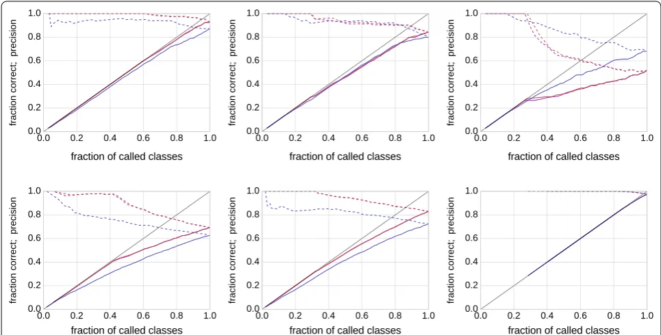
Figure 4 shows examples (the same as in Fig. 3) of the performance of each rule (rule 1: blue; rule 2: red; rule 3: magenta) in terms of N/n against C/n (fraction correct: solid) and C/N (precision: dashed). If a red or magenta curve is predominantly above the corresponding blue curve, using beta mixture modeling is advantageous for
this dataset. Mixture modeling fails in particular for the example in the upper right panel. Considering the cor-responding data in Fig. 3, the distribution is close to uniform except at the extremes, and indeed this is the prototypical case where beta mixtures do more harm than they help.
We are interested in the average performance over the simulated 1000 mixtures in dataset 1 (n=200) and data-set 2 (n=1000). As the magenta and red curve never dif-fered by much, we computed the (signed) area between the solid red and blue curve in Fig. 4 for each of the 1000 mixtures. Positive values indicate that the red curve (clas-sification by mixture modeling) is better. For dataset 1, we obtain a positive sign in 654/1000 cases (+), a nega-tive sign in 337/1000 cases (−) and absolute differences of at most 10−6 in 9/1000 cases (0). For dataset 2, the numbers are 810/1000 (+), 186/1000 (−) and 4/1000 (0). Figure 5 shows histograms of the magnitudes of the area between curves. While there are more instances with benefits for mixture modeling, the averages (−0.0046 for dataset 1; +0.0073 for dataset 2) do not reflect this because of a small number of strong outliers on the nega-tive side. Without analyzing each instance separately here, we identified the main cause for this behavior as close-to-uniformly distributed data, similar to the exam-ple in the upper right panel in Figs. 3 and 4, for which appropriate (but incorrect) parameters are found. In fact, a single beta distribution with α <0 and β <0 would
model is not well identifiable. Of course, such a situation can be diagnosed by computing the distance between the sample and uniform distribution, and one can fall back to fixed thresholds.
Simulation and fitting for estimating the number of components
To evaluate the component estimation algorithm, we simulate datasets with one to five components with
n=1000 samples. We simulate two different kinds of datasets, both using the method of picking the mixture coefficients π as described before.
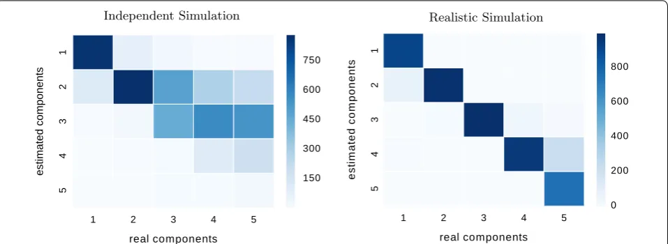
Independent simulation
For the dirst kind of data, we choose components inde-pendently from each other. This frequently leads to datasets that can be effectively described by fewer com-ponents than the number used to generate the dataset. Fig. 4 Performance of several classification rules. Shown is the fraction of called classes N/n (i.e., data points for which a decision was made) on the x-axis against the fraction of correct classes C/n (solid lines) and against the precision C/N (dashed lines) on the y-axis for three decision rules (blue: fixed intervals; red: highest weight with weight threshold; magenta: highest weight with gap threshold). The datasets are in the same layout as in Fig. 3
Let E be a standard exponentially distributed random variable with density function f(x)=e−x. The param-eters are chosen for each component j independently by choosing α=Ej,1 and β=1−Ej,2 from independent exponentials. (If β <0, we re-draw.)
Realistic simulation
We simulate more realistic and separable data by a sec-ond approach. The intention is to generate mixtures whose components are approximately equally distributed on the unit interval, such that each component slightly overlaps with its neighbors.
To generate a set of data points we pick an interval I = [E1, 1−E2] with exponentially distributed bor-ders. (If 1−E2<E1, or if the interval is too small to admit c components with sufficient distance from each other, we re-draw.) For each component j we uniformly choose a point µj∈I. We repeat this step if the dis-tance between any two µ values is smaller than 0.2. Sort the values such that E1< µ1<· · ·< µc<1−E2. Let dj:=min[{|µi−µj| :i�=j} ∪ {E1, 1−E2}]. Then we
set σj=1/4dj. Now µ and σ serve as mean and standard deviation for each component to generate its parameters αj and βj by Eq. (5).
Evaluation of component estimation
We estimate the number of components as described above with a dKS threshold corresponding to a p-value of ≥0.5 of the corresponding Kolmogorov–Smirnov test (as the fit becomes better with more components, the p-value is increasing). (The choice of 0.5 as a p-value threshold is somewhat arbitrary; it was chosen because it shows that there is clearly no significant deviation
between the fitted mixture and the empirical cdf from the data; see below for the influence of this choice.) We compare the true simulated number of components to the estimated number for 1000 datasets of 1000 points each, generated by (a) independent simulation and (b) realistic simulation. Figure 6 shows the resulting confu-sion matrix. Near-perfect estimation would show as a strong diagonal. We see that we under-estimate the num-ber of components on the independently generated data, especially for higher numbers of components. This is expected since the components of the independent sim-ulation often overlap and result in relatively flat mixture densities that cannot be well separated. For the data from the realistic stimualtions, we can see a strong diagonal: Our algorithm rarely over- or underestimates the num-ber of components if the components are separable. For both kinds of datasets, our method rarely overestimates the number of components.
Choice of p‑value threshold
In principle, we can argue for any “non-significant” p-value threshold. Choosing a low threshold would yield mixtures with fewer components, hence increase under-estimations but reduce overunder-estimations. Choosing a high threshold would do the opposite. By systematically varying the threshold we can examine whether there is an optimal threshold, maximizing the number of cor-rect component estimations. Figure 7 shows the fraction of both under- and overestimations for both datasets (I: independent, blue; R: realistic, brown), as well as the total error rate (sum of under- and overestimation rates) for varying p-value threshold. We see that the error rate is generally higher in the independent model (I) because we
Independent Simulation Realistic Simulation
systematically underestimate the true number of compo-nents (see above); this is true for any reasonable thresh-old ≤ 0.9. We also see that both total error curves have a flat valley between 0.4 and 0.6 (or even 0.2 and 0.8), so choosing any threshold in this range is close to optimal; we chose 0.5 because it is “least complex” in the sense of Occam’s Razor.
Discussion and conclusion
Maximum likelihood estimation in beta mixture mod-els suffers from two drawbacks: the inability to directly use 0/1 observations, and the sensitivity of estimates to ad-hoc parameters introduced to mitigate the first prob-lem. We presented an alternative parameter estimation algorithm for mixture models. The algorithm is based on a hybrid approach between maximum likelihood (for computing responsibility weights) and the method of moments; it follows the iterative framework of the EM algorithm. For mixtures of beta distributions, it does not suffer from the problems introduced by ML-only meth-ods. Our approach is computationally simpler and faster than numerical ML estimation in beta distributions. Although we established a desirable invariant of the sta-tionary points, other theoretical properties of the algo-rithm remain to be investigated. In particular, how can stationary points be characterized?
With a simulation study based on realistic param-eter settings, we showed that beta mixture modeling is often beneficial when attempting to infer an underlying single nucleotide variant state from observed methyla-tion levels, in comparison to the standard non-adaptive
threshold approach. Mixture modeling failed when the samples were close to a uniform distribution without clearly separated components. In practice, we can detect such cases before applying mixture models and fall back to simple thresholding.
We also showed that for reasonably separated com-ponents, our method often infers the correct number of components. As the log-likelihood is not available for comparing different parameter sets (the value would be ±∞), we used the surrogate Kolmogorov–Smirnov (KS) distance between the estimated cumulative distribu-tion funcdistribu-tion (cdf) and the empirical cdf. We showed that using any p-value threshold close to 0.5 for the cor-responding KS test yields both good and robust results. Under-estimation is common if the data has low com-plexity (flat histograms) and can be effectively described with fewer components.
A comparison of our algorithm with the EM algorithm (from the betareg package) failed because the EM algorithm did not converge and exited with errors (how-ever, we did not attempt to provide our own implementa-tion). We hope that our method will be widely adopted in the future for other problems involving beta mixtures because of its computational advantages, and we intend to further characterize its properties.
Authors’ contributions
SR had the idea to combine method-of-moments estimation with the iterative EM framework. CS provided the first implementation, designed and implemented the dynamic component estimation and performed simula-tion studies. Both CS and SR authored the manuscript. Both authors read and approved the final manuscript.
Acknowledgements
C.S. acknowledges funding from the Federal Ministry of Education and Research (BMBF) under the Project Number 01KU1216 (Deutsches Epigenom Programm, DEEP). S.R. acknowledges funding from the Mercator Research Center Ruhr (MERCUR), project Pe-2013-0012 (UA Ruhr professorship) and from the German Research Foundation (DFG), Collaborative Research Center SFB 876, project C1.
Competing interests
The authors declare that they have no competing interests.
Availability of data and materials
Data and Python code can be obtained from https://bitbucket.org/ genomeinformatics/betamix.
Consent for publication
Not applicable.
Ethics approval and consent to participate
Not applicable.
Publisher’s Note
Springer Nature remains neutral with regard to jurisdictional claims in pub-lished maps and institutional affiliations.
Received: 3 February 2017 Accepted: 8 August 2017 Fig. 7 Fraction of under- and overestimations and total error rate
• We accept pre-submission inquiries
• Our selector tool helps you to find the most relevant journal • We provide round the clock customer support
• Convenient online submission • Thorough peer review
• Inclusion in PubMed and all major indexing services • Maximum visibility for your research
Submit your manuscript at www.biomedcentral.com/submit
Submit your next manuscript to BioMed Central
and we will help you at every step:
References
1. Ji Y, Wu C, Liu P, Wang J, Coombes KR. Applications of beta-mixture mod-els in bioinformatics. Bioinformatics. 2005;21(9):2118–22.
2. Pounds S, Morris SW. Estimating the occurrence of false positives and false negatives in microarray studies by approximating and partitioning the empirical distribution of p-values. Bioinformatics. 2003;19(10):1236–42.
3. Dempster AP, Laird NM, Rubin DB. Maximum likelihood from incomplete data via the EM algorithm. J R Stati Soc Ser B. 1977;39(1):1–38. 4. Bury K. Statistical distributions in engineering. Cambridge: Cambridge
University Press; 1999.
5. Grün B, Kosmidis I, Zeileis A. Extended beta regression in R: shaken, stirred, mixed, and partitioned. J Stat Softw. 2012;48(11):1–25.
6. Redner RA, Walker HF. Mixture densities, maximum likelihood, and the EM algorithm. SIAM Rev. 1984;26:195–239.
7. Pearson K. Contributions to the mathematical theory of evolution. Philos Trans R Soc Lond A Math Phys Eng Sci. 1894;185:71–110.
8. Arthur D, Vassilvitskii S. K-means++: the advantages of careful seeding. In: Proceedings of the 18th annual ACM-SIAM symposium on discrete
algorithms. SODA ’07 society for industrial and applied mathematics, Philadelphia. 2007; pp. 1027–1035
9. Akaike H. A new look at the statistical model identification. IEEE Trans Autom Control. 1974;19(6):716–23.
10. Bhat H, Kumar N. On the derivation of the bayesian information criterion. Technical report, School of Natural Sciences, University of California, California; 2010
11. Massey FJ. The Kolmogorov–Smirnov test for goodness of fit. J Am Stat Assoc. 1951; 46(253): 68–78. Accessed 01 Dec 2016.
12. Adusumalli S, Mohd Omar MF, Soong R, Benoukraf T. Methodological aspects of whole-genome bisulfite sequencing analysis. Brief Bioinform. 2015;16(3):369–79.