A sub-cubic time algorithm for computing the quartet distance between two general trees

(1)

R E S E A R C H

Open Access

A sub-cubic time algorithm for computing the

quartet distance between two general trees

Jesper Nielsen

1,2*

, Anders K Kristensen

2

, Thomas Mailund

1

and Christian NS Pedersen

1,2

Abstract

Background:When inferring phylogenetic trees different algorithms may give different trees. To study such effects a measure for the distance between two trees is useful. Quartet distance is one such measure, and is the number of quartet topologies that differ between two trees.

Results:We have derived a new algorithm for computing the quartet distance between a pair of general trees, i.e. trees where inner nodes can have any degree≥3. The time and space complexity of our algorithm is sub-cubic in the number of leaves and does not depend on the degree of the inner nodes. This makes it the fastest algorithm so far for computing the quartet distance between general trees independent of the degree of the inner nodes.

Conclusions:We have implemented our algorithm and two of the best competitors. Our new algorithm is significantly faster than the competition and seems to run in close to quadratic time in practice.

Background

The evolutionary relationship between a set of species is conveniently described as a tree, where the leaves repre-sent the species and the inner nodes speciation events. Using different inference methods to infer such trees from biological data, or using different biological data from the same set of species, often yield slightly differ-ent trees. To study such differences in a systematic manner, one must be able to quantify differences between evolutionary trees using well-defined and effi-cient methods. One approach for this is to define a dis-tance measure between trees and compare two trees by computing this distance. Several distance measures have been proposed, e.g. the symmetric difference [1], the nearest-neighbour interchange [2], the subtree transfer distance [3], the Robinson and Foulds distance [4], and the quartet distance [5]. Each distance measure has dif-ferent properties and reflects difdif-ferent properties of the tree relationship.

For an evolutionary tree, the quartet topologyof four species is determined by the minimal topological subtree containing the four species. The four possible quartet topologies of four species are shown in Figure 1. Given

two evolutionary trees on the same set of nspecies, the

quartet distancebetween them is the number of sets of

four species for which the quartet topologies differ in the two trees.

Most previous work has focused on comparingbinary

trees and therefore avoided star quartets. Steel and Penny in [6] developed an algorithm for computing the quartet distance in time O(n3). Bryant et al. in [7] improved this result with an algorithm that computes the quartet distance in time O(n2). Brodalet al., in [8], presented the currently best known algorithm that algo-rithm the computes the quartet distance in time O(n

logn).

Recently, we have developed algorithms for computing the quartet distance between two trees of arbitrary

degrees, i.e. trees that can contain star quartets. In [9] we developed two algorithms: the first algorithm runs in time O(n3) and space O(n2)–and is thus independent of the degree of the inner nodes–the second in time O (n2d2) and space O(n2), whered is the maximal degree of inner nodes in the trees–and thus depends on the degree of the nodes. The O(n2d2) was later improved to O(n2d) [10], and by taking an approach similar to the Brodal et al.[8] O(nlogn) we developed a sub-quadra-tic algorithm in terms ofn but at a significant cost in terms ofd: O(d9nlogn) [11].

* Correspondence: [email protected] 1

Bioinformatics Research Centre (BiRC), Aarhus University, C. F. Møllers Alle 8, DK-8000 Aarhus C, Denmark

Full list of author information is available at the end of the article

(2)

In this paper we develop an O(n2+a) algorithm, where

α= ω−1

2 and O(n

ω_{) is the time it takes to multiply}

two n×n matrices. Using the Coppersmith-Winograd [12] algorithm, whereω = 2.376, this yields a running time of O(n2.688). The running time is thus independent of the degrees of the inner nodes of the input trees, and this is the first sub-cubic time algorithm with this prop-erty. Furthermore we have implemented the algorithm, along with two of the previous methods, and show experimentally that our new algorithm performs well in practice.

Methods: A sub-cubic time and space algorithm

The quartet distance between two trees is the number of quartets where the quartet topology differs between the two trees, i.e. the number of quartets where one tree has the star topology and the other a butterfly topology, plus the number of quartets where the trees have a different butterfly topology. As observed in [9], the former–where one tree has the star topology and the other a butterfly topology–can be expressed in terms of the total number of butter-flies in the two trees, the number of shared butterbutter-flies and the number of different butterflies: For trees T

and T’, the number of different topologies due to one being a star and the other a quartet, diffS(T, T’), is

given by

diffS(T,T) =B+B−2 (sharedB(T, T) + diffB(T,T)), (1)

whereBis the number of butterflies inT,B’the num-ber of butterflies in T’, sharedB(T, T’) the number of

quartets with the same butterfly topology inT and T’

and diffB(T’) the number of quartets with different

but-terfly topologies inT andT’. Thus the quartet distance betweenTand T’is given by the expression

qdist(T,T) =B+B−2sharedB(T,T)−diffB(T,T). (2)

Since,B= sharedB(T, T) andB’= sharedB(T’,T’), an

algorithm for computing sharedB(T,T’) and diffB(T, T’)

gives an algorithm for computing the quartet distance betweenTand T’.

Our approach to counting the shared and different quartets is based on directed quartetsand claims[8,9]. An (undirected) butterfly quartet topology, ab|cd

induces two directed quartet topologies ab® cd and

ab¬ cd, by the orientation of the middle edge of the topology, as shown in Figure 2. There are twice as many directed butterflies as undirected. Ife = (se,te) is

a directed edge fromsetotewe callsethe source ofe,

and tethe target. To each directed quartet, ab ® cd,

we can uniquely associate the directed edge, eso that

a and b are leaves in the subtree rooted at se, and c

and d are leaves in different subtrees rooted atte, see

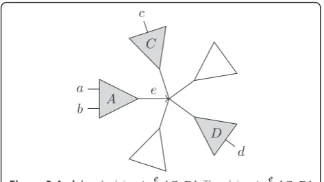
Figure 3. We call such a tree substructure, consisting of a directed edge e with a subtree, A behind e and two distinct subtrees, C and D, in front of e aclaim, written A→e (C,D). We say that the edge e claims the directed quartet ab® cd, and we also say that an edge

e claims an undirected quartetab|cd if it claims one of its directed quartets. Each (undirected) butterfly quar-tet defines exactly two directed butterfly quarquar-tets, and each directed quartet is claimed by exactly one direc-ted edge; considering each claim and implicitly each directed butterfly claimed by the claim, we can exam-ine each directed butterfly in a tree, or each undirected butterfly twice.

The crux of the algorithm is to consider each pair of claims, one from each tree, and for each such pair count the number of shared and different directed butterflies

a

b

c

d

Buttery ab|cd

a

c

b

d

Buttery ac|bd

a

d

b

c

Butteryad|bc

a

b

c

d

Star

Figure 1Quartet topologies. The four possible quartet topologies of speciesa, b, c, andd. For binary trees, only the butterfly quartets are possible.

a

b

c

d

(a)

a

b

c

d

(b)

a

b

c

d

(c)

(3)

claimed in the two trees. This way each shared butterfly is counted twice, and each different butterfly is counted four times, as shown in Figure 4. Dividing the counts by two and four, respectively, gives us sharedB(T, T’) and

diffB(T,T’).

Preprocessing

Before counting shared and different butterflies, we cal-culate a number of values in two preprocessing steps. First, we calculate a matrix that for each pairs of sub-treesF ÎT andGÎ T’stores the number of leaves in both trees, |F⋂ G|. This can be achieved in time and space O(n2) [7].

Next, for each pair of inner nodes, vÎ T, v’ÎT’with sub-treesFi,i= 1,...,dvandGj,j= 1, ...,dv’, respectively,

we calculate a matrix,I, such thatI[I,j] = |Fi⋂Gj|, and

we calculate vectors of its row and column sums, and the total sum of its entries:

R[i] =

dv

j=1

I[i,j] (3)

C[j] =

dv

i=1

I[i,j] (4)

M=

dv

i=1

dv

j=1

I[i,j] (5)

Inspired by the sums (S.3) - (S.6) in Additional file 1 we calculate a matrixI’, vectors of its row and column sums, the total sum of its entries, and some further values

I[i,j] =I[i,j](M−R[i]−C[j] +I[i,j]) (6)

R[i] =

dv

j=1

I[i,j] (7)

C[j] =

dv

i=1

I[i,j] (8)

M=

dv

i=1

dv

j=1

I[i,j] (9)

R[i] =

dv

j=1

I[i,j](C[j]−I[i,j]) (10)

A e

b a

D d C

c

Figure 3A claim. Aclaim _A→e ₍_C_,_D₎. The claim_A→e ₍_C_,_D₎ claims all ordered butterfliesab_®cdwherea, b_ÎAandc_ÎC,d

ÎDwhereCandDare twodifferentsubtrees in front ofe.

Shared

buttery directed claimsImplies two

T: a

b

c

d

T: a

b

c

d

=

Dierent

butterfy directed claimsImplies four

T: a

b

c

d

T: a

c

b

d

=

(4)

C[j] =

dv

i=1

I[i,j](R[i]−I[i,j]) (11)

R[i] =

dv

j=1

I[i,j]2 (12)

C[j] =

dv

i=1

I[i,j]2 (13)

Calculating the values in Eq. (3) - (13) can be done in O(dvdv’) for each pair of inner nodes (v, v’)Î T × T’,

giving a total time of

O

v∈T

v_∈Tdvdv

= O

v∈Tdv v_∈Tdv

= O(n2₎_.

Finally, we need to calculate the following values:

I[i,j] =

dv

k=1,k=i dv

l=1,l=j

I[i,l]I[k,j]I[k,l] (14)

which takes time O(d2vd2v) for each pair of inner nodes, giving a total time of O(n4), if done naively. However, as we show in section 1 of Additional file 1 the values in Eq. (14) can be calculated faster if we pre-compute either I₁=IIT_and _I

1 =I1I, or I2=ITI and

I₂ =II₂depending on which pair of matrices is fastest to compute, where I is the dv × dv’ matrix defined

above. We thus calculate either Eq. (15) and (16), or Eq. (17) and (18), depending on which pair is fastest to cal-culate.

I₁[i,k] =

dv

j=1

I[i,j]I[k,j] (15)

I₁ [i,j] =

dv

k=1

I[k,j]I₁[i,k] (16)

I₂[j,l] =

dv

i=1

I[i,j]I[i,l] (17)

I₂[i,j] =

dv

l=1

I[i,l]I₂[l,k] (18)

Calculating the values in Eq. (15) and (16) takes time O(max(dvdv)ω) if padding the matrices to become

square and with ω = 2.376 if using the Coppersmith-Winograd algorithm [12] for matrix multiplication, or timeO(d2

vdv)if using naive matrix multiplication.

Simi-larly, calculating the values in Eq. (17) and (18) takes time O(max(dvdv)ω)orO(dvd2v). Computing either I1

and I₁, or I₂ and I₂, thus takes time O(min(max(dv,dv)ω,d_v2dv,dvd2v)).

Counting shared butterfly topologies

For each pair of inner edges,eÎ Tande’ÎT’, see Fig-ure 5, we count the directed butterflies claimed by both

eande’. These are all on the form ab®cd, wherea,b ÎFi⋂Gj,cÎFk⋂GlanddÎFm⋂Gnfor some claims,

Fi e

→(Fk,Fm)and Gj e

→(Gl,Gn), of e and e’. The total number of directed butterflies common for bothe and

e’is therefore given by the expression 1

2

|Fi∩Gj|

2

k=i

l=j

|Fk∩Gl|

m=i,k

n=j,l

|Fm∩Gn| (19)

or the sum of1 2

I[i,j] 2

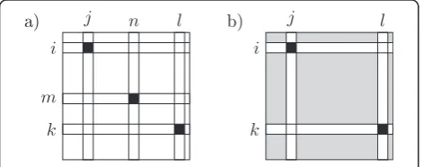
·I[k,l]·I[m,n]for all distinct entries in Ibut fixed (i,j), see Figure 6(a). We divide by two since we count each quartet twice, due to symmetry between the (k,l) and (m,n) pairs.

Notice, however, that the inner sum is simply the total sum of entries inI,M, except for the rowsi andkand columnsjand l, see Figure 6(b). Using

m=i,k

n=j,l

|Fm∩Gn|=M−

q=i,k

R[q]−

r=j,l

C[r] +

q=i,k

r=j,l

I[q,r] ₍₂₀₎

and the precomputed values we can, as shown in sec-tion 2 of Addisec-tional file 1 rewrite the expression in Eq. (19) to

1 2

I[i,j]

2

M−R[i]−C[j] +I[i,j]+

(I[i,j]−R[i]−C[j])(M−R[i]−C[j] +I[i,j])+

R[i]−I[i,j](C[j]−I[i,j])+

C[j]−I[i,j] (R[j]−I[i,j])

(21)

which can be computed in time O(1), if the referenced matrices have been precomputed. Thus we can compute all shared directed butterflies in total time O(n2). Divid-ing by two, we get the number of shared undirected butterflies.

Counting different butterfly topologies

Counting the number of different butterflies in the two trees is done similar to counting the number of shared butterflies. As before, we consider a pair of inner edges, eÎ T ande’Î T’. The quartets claimed by both

e and e’, but with different butterfly topology, are on the formaÎ Fi⋂ Gj, b ÎFi ⋂Gl, cÎ Fk⋂GjanddÎ Fm ⋂ Gn for some claims Fi

e

→(Fk,Fm) and Gj

e

(5)

|Fi∩Gj|

k=i

l=j

|Fi∩Gl||Fk∩Gj|

m=i,k

n=j,l

|Fm∩Gn|₍₂₂₎

or the sum ofI[I,j] ·I[I, l] ·I· [k,j]I[m,n] for all dis-tinct entries inIbut fixed (I,j), see Figure 7. In this case there is no need to divide by any normalizing constant, since there are no symmetries between k and m or betweenland n.

As before, the inner sum can be expressed as in Eq. (20), and using the precomputed values we can, as shown in section 3 of Additional file 1 rewrite the expression in Eq. (22) as

I[i,j](M−R[i]−C[j] +I[i,j])(R[i]−I[i,j])(C[j]−I[i,j])+

(R[i]−I[i,j])(I[i,j](R[i]−I[i,j])−C[j])+ (C[j]−I[i,j])(I[i,j](C[j]−I[i,j])−R[i])+

I1 [i,j]−I[i,j]I1[i,i]−I[i,j] (C[j]−I[i,j] 2

)

(23)

or

I[i,j](M−R[i]−C[j] +I[i,j])(R[i]−I[i,j])(C[j]−I[i,j])+

(R[i]−I[i,j]) (I[i,j](R[i]−I[i,j])−C[j])+ (C[j]−I[i,j]) (I[i,j](C[j]−I[i,j])−R[i])+

I2 [i,j]−I[i,j]I2[j,j]−I[i,j] (R[i]−I[i,j] 2

)

(24)

depending on whether we have precomputed I₁and I₁, orI₂andI₂. We can thus compute Eq. (22) in time O(1) for each pair of inner edgeseÎ Tande’ÎT’ giv-ing a total time of O(n2) to compute different directed, and thus different undirected, butterfly topologies in the two trees.

To get the actual number of different butterflies we have to divide by four.

Time analysis

The running time of the algorithm is dominated by the

time Omin (max (dv,dv)2.376,d2vdv,dvd2v)

it takes to

compute either I₁and I₁, orI₂andI₂, for each pair of nodesvÎ Tandv’ÎT’. Let O(nω) be the time it takes to multiply two n ×n matrices. In section 4 of Addi-tional file 1 we show that the running of our algorithm

is O(n2+a), whereα= ω−1

2 . Using the Coppersmith-Winograd algorithm [12] for matrix multiplication, whereω= 2.376, this yields a running time of O(n2.688).

Results

We have implemented our new algorithm and, for comparison, the O(n3) and O(n4) algorithms [9] for general trees. We chose those algorithm instead of those from [10,11], because the running time of those

Fi e

Fm Fk

Gj e

Gn Gl

Figure 5Comparing two edges. A pair of inner edges,eÎT,e’ÎT’, whereFi(Gj) is the sub-tree behinde(e’) andFk,k≠i(Gl,l≠j) the

remaining subtrees of the node pointed to bye(e’). Highlighted are two claims, one from each tree.

a)

i

m

k

j _n _l _b)

i

k

j _l

i

k

j _l

Figure 6Counting shared quartets. Graphical illustration of the shared quartet expression, eq. (19). On the left, the matrix entries summed over are explicitly shown. On the right, the inner sum is implicitly shown. The sum of the greyed entries can be computed in constant time.

a)

i

m

k

j _n _l _b)

i

k

j _l

i

k

j _l

(6)

algorithms are dependent on the degree of the nodes, while a major feature of our new algorithm is that it has a good asymptotical running time independent of the degree of the nodes. For matrix multiplication we link to a BLAS library, and expect that to choose the most efficient algorithm for matrix multiplication. In our experiments the vecLib library from Mac OS X is used. We have run benchmarks with trees with ten leaves up to trees with almost 15, 000 leaves. For each size, trees were generated in four different ways: gen-eral trees, binary trees, star trees and trees with one

node of degree n

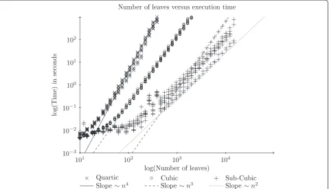
2 surrounded by degree 3 nodes. The code that generated the trees is available in Additional file 2. For each of the ten possible combinations of topologies, one pair of trees were randomly generated, and the time used for the computation of the quartet distance was measured and plotted. Our experiments were run on a Mac-Pro with two Intel quad-core Xeon processors running at 2.26 GHz and with 8 GB RAM. As seen in Figure 8 the implementation of our new algorithm is significantly faster than the implementa-tions of the competing algorithms, on trees with many leaves. In the worst cases our algorithm approaches O

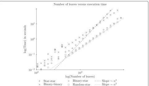
(n3) which is expected if the BLAS implementation uses the O(n3) matrix multiplication algorithm. Indeed Figure 9 shows that the slowest of our runs are on two star-shaped trees, where we need to multiply two n×

n matrices and where the time-complexity of the matrix multiplication algorithm is most important. However, in most cases our algorithm seems to be close to quadratic execution time, even though it apparently uses an asymptotically slow matrix multipli-cation algorithm.

Conclusion

We have derived, implemented and tested a new algo-rithm for computing the quartet distance. In theory our

algorithm has execution time O(na+2), where_α= ω−1 2 . With current knowledge of matrix multiplication this is O(n2.688). If an algorithm for matrix multiplication in time O(n2) is found this would make our algorithm run in time O(n2.5). Experiments on our implementation shows it to be fast in practice, and that it can have a running time significantly better than the theoretical upper bound, depending on the topology of the trees being compared.

× Quartic ◦ Cubic + Sub-Cubic

Slope ∼n4 Slope∼n3 Slope∼n2

Number of leaves versus execution time

log(Number of leaves)

101 ₁₀2 ₁₀3 ₁₀4

log(Time)

in

seconds

10−3

10−2

10−1

100 101 102 ◦◦◦◦◦◦ ◦◦◦ ◦ ◦◦◦◦ ◦◦ ◦◦ ◦◦ ◦◦ ◦◦ ◦◦ ◦◦ ◦◦ ◦◦◦◦◦◦ ◦◦◦ ◦ ◦◦ ◦◦◦ ◦◦ ◦◦ ◦◦ ◦◦ ◦◦ ◦◦ ◦◦ ◦ ◦◦◦◦◦◦ ◦◦◦◦◦ ◦◦◦ ◦◦ ◦◦ ◦◦ ◦◦ ◦◦ ◦◦ ◦◦ ◦ ◦◦◦◦◦◦ ◦◦◦◦◦ ◦◦◦ ◦◦ ◦◦◦ ◦◦ ◦◦ ◦◦ ◦◦ ◦◦ ◦ ◦◦◦◦◦◦ ◦ ◦◦◦◦ ◦◦◦ ◦◦ ◦◦◦ ◦◦ ◦◦ ◦◦ ◦◦ ◦◦ ◦ ◦◦◦◦◦◦ ◦◦◦ ◦ ◦◦ ◦◦ ◦◦ ◦◦ ◦◦ ◦◦ ◦◦ ◦◦ ◦◦ ◦ ◦◦◦◦◦◦ ◦ ◦◦◦◦ ◦◦◦ ◦◦ ◦◦◦ ◦◦ ◦◦ ◦◦ ◦◦ ◦◦ ◦ ◦◦◦◦◦◦ ◦◦◦ ◦ ◦◦ ◦◦ ◦◦ ◦◦ ◦◦ ◦◦ ◦◦ ◦◦ ◦◦ ◦ ◦◦◦◦◦◦ ◦◦◦◦◦ ◦◦ ◦◦ ◦◦ ◦◦ ◦◦ ◦◦ ◦◦ ◦◦ ◦◦ ◦◦◦◦◦◦ ◦ ◦◦◦◦ ◦◦ ◦◦ ◦◦ ◦◦ ◦◦ ◦◦ ◦◦ ◦◦ ◦◦ ××××× ×× ×× ×× ×× ×× ×× ×× × ×××× ×× ×× ×× ×× ×× ×× ×× ×× ××××× ×× ×× ×× ×× ×× ×× ×× ×× ××××× ×× ×× ×× ×× ×× ×× ×× ×× ×××× ×× ×× ×× ×× ×× ×× × ×× ×× ××××× ×× ×× ×× ×× ×× ×× ×× ×× ×××× ×× ×× ×× ×× ×× ×× × ×× ×× ×××× ×× ×× ×× ×× ×× ×× × ×× ×× ×××× ×× ×× ×× ×× ×× ×× × ×× ×× ××××× ×× ×× ×× ×× ×× ×× ×× ×× +++++++++ ++++++ +++ +++++ ++++ ++++ ++++ ++ ++ +++++++++++++ ++++ +++ + ++++ ++++ ++++ ++++ ++ + + +++++++ + ++++++ + + + + + ++++ ++++ +++ ++++ +++ ++ +++++++++++++ ++++ + + + + ++++ ++++ ++++ +++ +++ + + + +++++++++++ +++++ + + + ++++ ++++ ++++ +++ +++ + +++++++++++++++ +++ + + + +++++ ++++ ++++ +++ ++++ +++++++++++++++ +++ + + + ++++ ++++ +++ ++++ ++++ +++++++++++ + +++ +++ + + + +++ ++ ++ ++ ++ ++ ++ ++ + +++++++++ + +++++++ + + + + ++++ ++++ +++ ++ ++ ++ ++ + +++++++++++++++ +++ + + + ++++ ++++ ++++ ++++ ++ ++

Figure 8Comparison of algorithms. Plotted are our new algorithm compared to previously known O(n3_{) and O(}_n4_{) algorithms. In a log-log} plotxb_{becomes a straight line with the slope determined by}_b_{. The lines in the plot are not regression lines, but are inserted to help the}

(7)

Availability

The software is available from http://www.birc.au.dk/ software/qdist. It has been tested on Ubuntu Linux and Mac OS X.

Additional material

Additional file 1: Supplementary material containing mathematical derivations that are too tedious for the main text.

Additional file 2: The python script used to generate the random trees for the experiments.

Acknowledgements

We are grateful to Chris Christiansen, Martin Randers and Martin S. Stissing for many fruitful discussions about the quartet distance.

Author details 1

Bioinformatics Research Centre (BiRC), Aarhus University, C. F. Møllers Alle 8, DK-8000 Aarhus C, Denmark.2_{Department of Computer Science, Aarhus} University, Åbogade 34, DK-8200 Aarhus N, Denmark.

Authors_’contributions

JN, TM and CP developed the algorithm. AK implemented the algorithm. AK and JN benchmarked and evaluated the algorithm. JN, TM and CP wrote the paper. All authors read and approved the paper.

Competing interests

The authors declare that they have no competing interests.

Received: 12 April 2011 Accepted: 3 June 2011 Published: 3 June 2011

References

1. Robinson DF, Foulds LR:Comparison of weighted labelled trees.

Combinatorial mathematics, VI (Proc. 6th Austral. Conf), Lecture Notes in Mathematics, Springer1979, 119-126.

2. Waterman MS, Smith TF:On the similarity of dendrograms.Journal of Theoretical Biology1978,73:789-800.

3. Allen BL, Steel M:Subtree transfer operations and their induced metrics on evolutionary trees.Annals of Combinatorics2001,5:1-13.

4. Robinson DF, Foulds LR:Comparison of phylogenetic trees.Mathematical Biosciences1981,53:131-147.

5. Estabrook G, McMorris F, Meacham C:Comparison of undirected phylogenetic trees based on subtrees of four evolutionary units.Syst Zool1985,34:193-200.

6. Steel M, Penny D:Distribution of tree comparison metrics-some new results.Syst Biol1993,42(2):126-141.

7. Bryant D, Tsang J, Kearney PE, Li M:Computing the quartet distance between evolutionary trees.Proceedings of the 11th Annual Symposium on Discrete Algorithms (SODA)2000, 285-286.

8. Brodal GS, Fagerberg R, Pedersen CNS:Computing the Quartet Distance Between Evolutionary Trees in TimeO(nlogn).Algorithmica2003,38:377-395. 9. Christiansen C, Mailund T, Pedersen CNS, Randers M:Algorithms for

Computing the Quartet Distance between Trees of Arbitrary Degree.

Proc. of Workshop on Algorithms in Bioinformatics (WABI), Volume 3692 of Lecture Notes in Bioinformatics (LNBI), Springer-Verlag2005, 77-88. 10. Christiansen C, Mailund T, Pedersen CNS, Randers M, Stissing MS:Fast

calculation of the quartet distance between trees of arbitrary degrees.

Algorithms for Molecular Biology2006,1.

11. Stissing M, Pedersen CNS, Mailund T, Brodal GS, Fagerberg R:Computing the quartet distance between evolutionary trees of bounded degree.In

Proceedings of the 5th Asia-Pacific Bioinfomatics Conference 2007, Volume 5 of Series on Advances in Bioinformatics and Computational BiologyEdited by: Sankoff D, Wang L, Chin F 2007, 101-110.

+ Star-star

× Binary-binary ◦ Binary-starRandom-star

Slope∼n3

Slope∼n2

Number of leaves versus execution time

log(Number of leaves)

102 ₁₀3

log(Time)

in

seconds

10−2

10−1

100

101

+ + + +

+ +

+ + + +

++ ++

++ +

◦ ◦

◦ ◦ ◦

◦ ◦ ◦ ◦

× ××

× ×

×

×× ×

××

× × ×

Figure 9Comparison of tree topologies. This plot shows the two best and the two worst pairs of tree topologies, for our new algorithm only. In a log-log plotxb_{becomes a straight line with the slope determined by}_b_{. The lines in the plot are not regression lines, but are inserted}

(8)

12. Coppersmith D, Winograd S:Matrix multiplication via arithmetic progressions.Journal of Symbolic Computation1990,9:251-281.

doi:10.1186/1748-7188-6-15

Cite this article as:Nielsenet al.:A sub-cubic time algorithm for computing the quartet distance between two general trees.Algorithms for Molecular Biology20116:15.

Submit your next manuscript to BioMed Central and take full advantage of:

• Convenient online submission

• Thorough peer review

• No space constraints or color figure charges

• Immediate publication on acceptance

• Inclusion in PubMed, CAS, Scopus and Google Scholar

• Research which is freely available for redistribution