Discovery of Hidden Temporal Patterns in Earthquakes Data
Sohair F. Higazi
Professor of Statistics
Faculty of Commerce, Tanta University [email protected]
Rania M. Shalaby
Assistant Lecturer of Statistics
The Higher Institute for Managerial Science, Egypt [email protected]
Walaaeldien Abdelhadi
Principal Service Delivery Manager Oracle Corporation
Abstract
Time Series Data mining (TSDM) is one of the most widely used technique that deals with temporal patterns. Genetic algorithm (GA) is a predictive TSDM search technique that is used for solving search/optimization problems. GA is based on the principles and mechanisms of natural selections to find the most nearest optimal solution available from a list of solutions. GA relies on a set of important fundamentals, such as chromosome, crossover and mutation. GA is applied to earthquakes data in the year 2003-2004 in the Suez Gulf in Egypt, gathered from the Egyptian National Seismic Network. The study does not aim to building time series models from the point of time, since the analysis neither include the time nor the prediction of when an earth quake will occur, but to determine the possibility of occurrence of a strong magnitude earthquake after specific sequence of previous earthquakes as temporal pattern. The temporal pattern cluster used is a "circle". The objective function used is a function that gives the highest percentage of correct classification. Empirical results show that crossover and mutation probabilities are 0.4 and .01 respectively for both the training and the testing sample. The algorithm yields 96.98% correct classification for the training sample, and 95.35% for the testing sample.
Keywords: Temporal Patterns, TSDM, Genetic Algorithm (GA), Fitness Function,
Temporal Pattern Cluster.
Introduction
Time series data suffers, in many applications, of being unobvious, chaotic, hidden and non-periodic. Traditional time series analysis methods are limited by the requirement of stationary of the time series and normality and independence of the residuals. When these assumptions are not satisfied, traditional time series techniques yield inaccurate results. Time Series Data Mining (TSDM) techniques overcome the violation of these assumptions and help to discover important hidden patterns in the data.
Guide"). DM has two main functions: descriptive data mining via decision trees and neural networks (Feng and Povinelli 2003), and predictive data mining via Genetic algorithm, genetic programming, regression and correlation analysis, discriminant analysis, cluster analysis, and generalized Linear Models (El-Telbany 2004; Hui 2003). DM has been used in many disciplines, to name a few, marketing, direct Marketing, tourism marketing, finance applications, pharmaceutical industries, retailing; and also it has been used to investigate disease risks and health care.
In data mining sample data is partitioned into two sets: a "training set" and a "testing set". The training set is used to "train" the data mining algorithm, while the testing set is used to verify the accuracy of any patterns found.
Time Series Data Mining (TSDM) is an integration of several methods such as cluster analysis, time series analysis and machine language (Genetic Algorithm, and non-linear systems). The TSDM framework has the ability to overcome the shortcomings of traditional time series analysis. Genetic algorithm (GA) is one of the most widely used techniques that deal with temporal patterns; it aims to extract hidden information from numerous databases that practically would be difficult to identify significant events. GA is a predictive data mining technique that is used for solving search/optimization problems. GA is based on the mechanisms of natural selections, such as chromosome, crossover and mutation to find the most nearest optimal solution available from a list of solutions.
Genetic algorithm (GA), was inspired by Darwin's evolution theory, first introduce by Holland (1975), and then used in many applications (Povinelli 2000, 2001, 2003; Koza 1992; Alata et al. 2008; Feng and Povinelli 2003). GA uses cluster analysis to discover temporal patterns (hidden structures in time series data) to reach optimal solution to complex problems, it "characterizes" events to be able to "predict" them. Events such as earthquakes, volcanoes, flooding, and wilderness fires do happen over time, but they cannot be looked at as time series since they are "unpredictable". Such events have hidden structures (temporal patterns) and should be treated as "independent events", or to possibly be related to the occurrence of a "specific sequence of previous events".
GA and genetic programming were used in many applications; Povinelli and Feng (2003) used GA as an identification method for the characterization and prediction of complex time series events; they have used it to predict metal droplet release events during the welding process. Povinelli and Duan (2001) used genetic programming to estimate stock market prices by applying a TSDM framework; Povinelli and Diggs (2003) used GA to predict weekly financial time series; and was used by El-Telbany (2004) to predict the Egyptian stock market return.
scale magnitude more than the upper hinge of Box Plot diagram for the training sample data, and then apply the obtained classification algorithm on the testing sample data, to reach a specific sequence of previous earthquakes as a temporal pattern for an earthquake to be considered as an outlier of high magnitude.
Section 1introduces time series data mining; genetic algorithm (GA) is presented in Section 2; the methodology followed is given in Section 3; results are shown in Section 4, and conclusions are given in Section 5.
1. Time Series Data Mining (TSDM)
Traditional time series analysis methods assume stationarity of the time series, normality and independence of errors. Traditional time series analysis methods are unable to identify complex (non-periodic, nonlinear, irregular, and chaotic) characteristics. TSDM methods overcome the limitations of traditional time series analysis techniques; it helps to discover important hidden patterns in the data.
We distinguish here between some basic definitions used in TSDM (Povinelli 1999): a. Temporal Pattern is a hidden structure in time series data. It is used to"
characterize" an event to be able to predict it. The temporal Pattern P is a real vector of length "Q", expressed within the lagged time series with a point as:
Q
R
p
Where:
R
Q is the set of real numbers in the series regardless of time with Q dimension.The following graph shows the "event" and the temporal pattern:
Where;xtis the observation at time t,dark squares are events, and bright squares are
the temporal patterns (Povinelli 1999).
c. Time Delayed Embedded: a time series is transformed to a time-lagged series that gets rid of "time" called "Phase Space". It is a Q dimensional series that depends on the length of the temporal pattern. If Q =2, the time delayed embedded series take the value of xt and xt-1, thus two points are used, the value at time t and the
preceding value at timet-1, in this situation, the time lag =1.
d. Event Characterization Function: is a link between two temporal patterns; this link depends on the event to be characterized, and differs according to the type of event and the objective function of the data mining algorithm. When discovering a future one-time unit event, the characterization function is: g(t) x t1, and when
discovering a future event from more than three-time units' event, the objective function is:
g
(
t
)
max
{
x
t1,
x
t2,
x
t3}
e. Objective Function: Genetic Algorithm assigns the optimal solution from all feasible solutions. The objective function depends on the application area and the objective of the study. The objective function may take a form of a t-test to test if the mean points in the temporal pattern cluster equals to the mean points outside the cluster (Povinelli 1999), reaching a maximum predictive accuracy, sensitivity, specificity function, …etc. .
2. Genetic Algorithm (GA)
GA is a new method for analyzing time series data; it employs time-delayed embedding and identifies temporal patterns in the resulting phase spaces. GA provides efficient, effective techniques for optimization and machine learning applications; it is widely-used today in business, scientific and engineering disciplines. In GA, an optimization method is applied to search the phase spaces for optimal heterogeneous temporal pattern clusters that reveal hidden temporal patterns, which are characteristic and predictive of time series events (Povinelli and Feng 2003). The target is to reach the optimal solution to an "objective function", also called "fitness functions" (Beasley et al. 1993). GA uses same terminologies and basics used in evolution theory, namely: chromosome, crossover and mutation, defined as follows:
a. A chromosomerepresents the possible feasible solutions to a problem (Beasley et
al 1993). In GA, chromosomes need to be encoded. There are several encoding methods depending on the problem to be solves. There are binary encoding (the most widely used), where every chromosome is a string of bits 0 or 1; there is permutation encoding, which is useful for ordering problems; there is value encoding, where every chromosome is a string of some values that are connected to the problem; and there is tree encoding, where every chromosome is a tree of some objects or functions.
b. Crossover combines (mates) two chromosomes (parents) to produce a new
chromosome (offspring). The idea behind crossover is that the new chromosome may be better than both of the parents if it takes the best characteristics from each of the parents. Crossover occurs during evolution according to a user-definable crossover probability.
c. Mutation alters one or more gene values in a chromosome from its initial state.
solution than was previously possible. It occurs during evolution according to a user definable probability, usually is set very low (0.01).
GA then works in a following way. In every generation, select a few (good - with high fitness) chromosomes (solutions) for creating a new offspring (solution). Then some (bad - with low fitness) chromosomes (solutions) are removed and the new offspring is placed in their place. The rest of population survives to new generation.
For each new solution to be produced, a pair of "parent" solutions is selected for breeding from the pool selected previously. By producing a "child" solution using the above methods of crossover and mutation, a new solution is created which typically shares many of the characteristics of its "parents". New parents are selected for each new child, and the process continues until a new population of solutions of appropriate size is generated. These processes ultimately result in the next generation population of chromosomes that is different from the initial generation. Some off springs (solutions) may be selected as "elites" or best chromosome to new population. The rest is done in classical way. Elitism can rapidly increase performance of GA, because it prevents losing the best found solution. This is repeated until some condition (for example number of populations or improvement of the best solution) is satisfied.
Thus;
- Reproduction is selecting randomly a set of optimal solutions, and then mutates them and selects the best solution.
- Cross over: produce a new set of feasible solutions to form new offspring (new solution).
- Mutation: mutate new offspring at each position in chromosome.
- Conversion: approaching uniformity and stability to reach Global Optimum.
The main parameters of GA are the implementation of crossover and a fitness factor. Fitness factor means assigning a value (a probability) to one or more strings as being a better solution than other strings that result from reproduction, crossover and mutation.
3. Methodology
Time series data used for training purposes phase, takes the following form:
}
,...,
1
,
{
x
t
N
X
t
The second phase run is to choose a testing group of the time series, such that:
N
S
R
S
R
t
x
Y
{
t,
,...,
}
The event is characterized as:
g (t ) = { xt+1│xt, xt-1}
not take time into consideration. For each observation at time (t), there is always xt-1, xt
and xt+1. Box plot is used for the inspection of the xt+1values, to check for outliers. The
xt+1were coded to classify events and non-events as shown below:
event no otherwise
event hinge
upper x
if
x t
t 0
1 1
1
1
t
x are used as a binary classifier for clustering.
MATLAB, Genetic Algorithm procedure was used. The temporal pattern is defined as a circle, the objective function, the optimization formulations and constraints used in the GA procedure are given below.
Sandikci (2000) gave the steps Genetic Algorithm follows; this includes defining the number of chromosomes, fitness value for each solution, choice of new population: elite selections, crossover and mutation probabilities, replacing a solution into a newer one, and testing to know when to stop. Some parameters also have to be defined in the algorithm (Mathworks 2004); such as defining the fitness function, generations, population size, elite counts, best fitness value, selection options, and stopping conditions.
The objective function used in the study is a function that maximizes prediction accuracy by giving the percentage of accurate classification (Povinelli and Feng 2003), as follows:
n p n p
n p
f f t t
t t C
f
)
( (1)
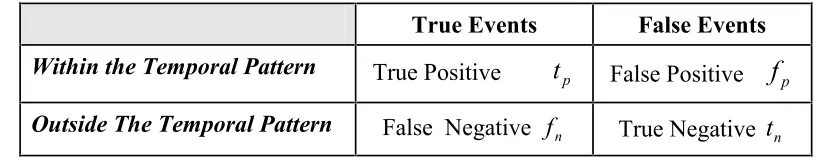
Where; tp: are the true positive events; tn is the True Negative events; fp is the False
Positiveevents, and fnis the number of FalseNegative events, as shown in the following
Table:
Table 1: Classification Table
True Events False Events
Within the Temporal Pattern True Positive tp False Positive
f
pOutside The Temporal Pattern False Negative fn True Negative tn
The function that minimizesfalse positives is:
p p
p f t
t C
f( ) (2)
is used to find one single temporal pattern cluster. Also, true positivepercentage is called sensitivity rate, found according to the formula:
n p
p f t
t C
True negativespercentage is called "Specificity rate" obtained according to the formula: p n n f t t C
f( ) (4)
Genetic algorithm is applied on the training group, using combinations of the following crossover and mutation probabilities:
Crossover: 0.2, 0.4, 0.6 and 0.8 Mutation: 0.01, 0.02, and 0.03
The best combination of crossover and mutation is reached for the temporal pattern; prediction accuracy, specificity and sensitivity measures are computed for the training set, and then applied to the testing group (Povinelli 2000).
4. Results
Data used are from Egyptian National Seismic Network, covering earth quakes data in several areas in the country for the year 2003-2004. Data included time, date, magnitude (in Richter scale), longitude, latitude, and depth from sea water level. The purpose is to reach the temporal pattern, where we can classify the magnitude in any particular time as a function of the magnitude of the previous magnitudes.
The Latitude and longitude are used to classify active zones, the Suez Gulf zone data is chosen for the analysis. Data for the second quarter of 2004 is chosen as a training group, and data for the third quarter of the year is chosen as the "testing group". Figure 1 gives a
time series line graph of the magnitude of training set (n=332), Figure 2 gives a time series line graph for the testing set (n=452).
Magnitude -1 -0.5 0 0.5 1 1.5 2 2.5 3 3.5 4 20 04 -4 -1 -1 2: 18 20 04 -4 -7 -1 6: 2 20 04 -4 -1 2-17 :5 1 20 04 -4 -1 6-21 :2 0 20 04 -4 -2 1-1: 8 20 04 -4 -2 5-13 :2 6 20 04 -4 -2 7-16 :2 1 20 04 -4 -2 9-2: 46 20 04 -5 -3 -1 8: 21 20 04 -5 -6 -2 1: 46 20 04 -5 -1 1-11 :4 3 20 04 -5 -1 5-1: 13 20 04 -5 -1 9-6: 43 20 04 -5 -2 5-18 :1 20 04 -5 -2 7-14 :1 0 20 04 -5 -3 0-2: 48 20 04 -6 -3 -1 0: 47 20 04 -6 -1 1-9: 58 20 04 -6 -1 2-23 :5 1 20 04 -6 -1 8-2: 50 20 04 -6 -1 9-11 :1 20 04 -6 -2 2-3: 33 20 04 -6 -2 6-0: 46 20 04 -6 -2 8-1: 42 Magnitude Magnitude -1 -0.5 0 0.5 1 1.5 2 2.5 3 3.5 4 20 04 -4 -1 -1 2: 18 20 04 -4 -7 -1 6: 2 20 04 -4 -1 2-17 :5 1 20 04 -4 -1 6-21 :2 0 20 04 -4 -2 1-1: 8 20 04 -4 -2 5-13 :2 6 20 04 -4 -2 7-16 :2 1 20 04 -4 -2 9-2: 46 20 04 -5 -3 -1 8: 21 20 04 -5 -6 -2 1: 46 20 04 -5 -1 1-11 :4 3 20 04 -5 -1 5-1: 13 20 04 -5 -1 9-6: 43 20 04 -5 -2 5-18 :1 20 04 -5 -2 7-14 :1 0 20 04 -5 -3 0-2: 48 20 04 -6 -3 -1 0: 47 20 04 -6 -1 1-9: 58 20 04 -6 -1 2-23 :5 1 20 04 -6 -1 8-2: 50 20 04 -6 -1 9-11 :1 20 04 -6 -2 2-3: 33 20 04 -6 -2 6-0: 46 20 04 -6 -2 8-1: 42 Magnitude
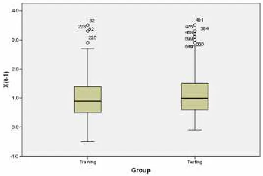
Box Plot for both groups is given in Figure 3 on xt-1, where it is evident that magnitudes
more than 2.9 Richter is considered an extreme value, observed values show 4 extreme earthquakes in the training sample and 7 in the testing sample.
Figure 3:Box Plot for earthquakes magnitude for xt-1
Povinelli (2000) recommends changing the time series into a phase space observations, thus; x t1 and x t1 are created from the time series data. A non-significant test of
equality on means is found, (α=0.05) between the testing and the training groups on xt , 1
t
x and x t1 .
Thus, an event (strong magnitude) is defined as follows:
event no otherwise
event x
if
x t
t 0
9 . 2
1 1
1
A "circle" is chosen to represent the temporal pattern cluster. A time delayed embedded with vector dimension Q=2 is chosen; thus, the xt-1 is the first dimension, and xt is the
second dimension; adding the link function g(t)= xt+1we get a third dimension, and the
optimal temporal pattern cluster is sought
Trial and error processes were followed using MATLAB GA tool. The optimal solution that maximizes the objective function of interest is found when using the following parameters:
- Population type:Real vector, which means using the real values ofxt.
- Initial range for the temporal pattern cluster (circle) is the range between 0 and 1. - Population size (number of solutions) = 50.
- Elite count=2.
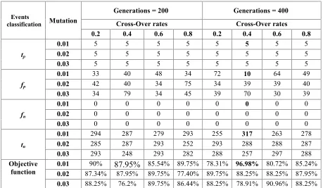
Results for the training group are shown in Table 2. It is found that the temporal circle cluster, at crossover rate=0.02, mutation rate =0.01 and generations=200 achieved an optimal solution of the objective function, with predictive accuracy = 90%, the number of true positives within the cluster, tpis 5; the number of false positive is 33. Increasing the
number of iteration to 400, at crossover rate=0.4 and mutation rate =0.01, the prediction accuracy increases to 96.98% with 5 true positive and 10 false positive events. The sensitivity, Eq. [3], and the specificity, Eq. [4], rates are 100% and 96.94% respectively.
Table 2: Objective function for different crossover and mutation rates, for 200 and 400 generations (Training Group)
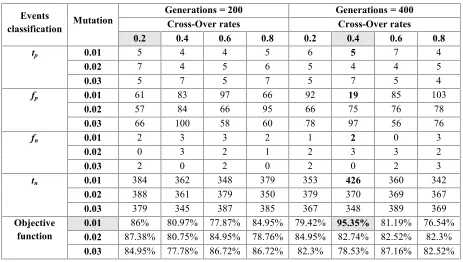
Using results obtained from the training group, where the number of iterations = 400, crossover rate=0.4 and mutation rate =0.01 yields a prediction accuracy (Eq. [1]) of 95.35% with 5 events classified as true positive and 19 events classified as false positive. The true positive percentage or the sensitivity rate (Eq. [3]) for the testing group is (5/7*100) = 71.42% and the true negative percentage or the specificity rate (Eq. [4]) is (426/445)*100= 95.73%.
MATLAB produces the optimal temporal cluster, which is a circle with, maximum number to be contained in the temporal pattern = 5.9548 earthquakes with magnitude more than 2.9 Richter, and the temporal pattern cluster were not able to reach 6 events. The radius of the circle is δ= 0.5043, centered at{x= =1.2183} and {y = =1.4897}. Thus, for an earthquake to be more than 2.9 Richter in time (t+1), the magnitude at time (t-1) to range between {δ ± 1.2183}, i.e. from {0.71 to 1.72} on the Richter scale, and the magnitude at time t to range between {δ ± 1.4897}, i.e. from {1 to 1.98} on the Richter scale, with prediction accuracy 95.35%.
Events
classification Mutation
Generations = 200 Generations = 400 Cross-Over rates Cross-Over rates 0.2 0.4 0.6 0.8 0.2 0.4 0.6 0.8
tp
0.01 5 5 5 5 5 5 5 5
0.02 5 5 5 5 5 5 5 5
0.03 5 5 5 5 5 5 5 5
fp
0.01 33 40 48 34 72 10 64 49
0.02 42 40 34 75 34 39 39 40
0.03 34 79 34 45 39 70 30 39
fn
0.01 0 0 0 0 0 0 0 0
0.02 0 0 0 0 0 0 0 0
0.03 0 0 0 0 0 0 0 0
tn
0.01 294 287 279 293 255 317 263 278
0.02 285 287 293 252 293 288 288 287
0.03 293 248 293 282 288 257 297 288
Objective
Testing phase run is performed on the testing group data using the temporal pattern cluster reached during the training stage. Table 3 gives the results of crossover and mutation probabilities using the same parametric values for the training group, and for generations 200 and 400.
Table 3: Objective function for different crossover and mutation rates, for 200 and 400 generations (Testing Group)
5. Conclusions
Genetic algorithm is applied to earthquakes data for the year 2003-2004 in the Suez Gulf in Egypt, gathered from the Egyptian National Seismic Network. The objective of the study was not building a time series models from the point of time, since the analysis neither includes the time nor the prediction when an earthquake will occur, but to determine the possibility of occurrence of a strong earthquake (event) after specific sequence of previous earthquakes as temporal pattern.
The temporal pattern cluster used is a "circle"; the objective function chosen is a function that gives the highest percentage of correct classification. Empirical results show that for the training sample, the crossover and mutation probabilities that satisfy the objective function are 0.4, and .01 respectively; these probabilities yield 96.98% correct classification. Applying the same crossover and mutation probabilities (0.4 and .01) on the testing sample, the obtained correct classification is 95.35%. This means that the genetic algorithm procedure was efficiently able to analyze and classify chaotic and non-stationary data in a significant way.
Events
classification Mutation
Generations = 200 Generations = 400 Cross-Over rates Cross-Over rates
0.2 0.4 0.6 0.8 0.2 0.4 0.6 0.8
tp 0.01 5 4 4 5 6 5 7 4
0.02 7 4 5 6 5 4 4 5
0.03 5 7 5 7 5 7 5 4
fp 0.01 61 83 97 66 92 19 85 103
0.02 57 84 66 95 66 75 76 78
0.03 66 100 58 60 78 97 56 76
fn 0.01 2 3 3 2 1 2 0 3
0.02 0 3 2 1 2 3 3 2
0.03 2 0 2 0 2 0 2 3
tn 0.01 384 362 348 379 353 426 360 342
0.02 388 361 379 350 379 370 369 367
0.03 379 345 387 385 367 348 389 369
Objective
function 0.010.02 87.38% 80.75% 84.95% 78.76% 84.95% 82.74% 82.52%86% 80.97% 77.87% 84.95% 79.42% 95.35% 81.19% 76.54%82.3%
References
1. Alata Mohanad, Molhim Mohammed and Ramni Abdullah (2008). "Optimizing of Fuzzy C-Means Clustering Algorithm Using GA". PWASER Vol. 29, pp. 224-229.
2. Beasley David, Bull David and Martin Ralph (1993). "An Overview of Genetic Algorithm: Part 2, Research Topics". University Computing 15(2), pp. 58-69. 3. El-Telbany Mohammed E. (2004). "The Egyptian Stock Market Return
Prediction: A Genetic Programming Approach", IEEE Computer Society, pp. 161-164.
4. Holland, John H. (1975).Adaptation in Natural and Artificial Systems, University of Michigan Press, Ann Arbor
5. Hui, Anthony (2003). "Using Genetic Programming to Perform Time Series Forecasting of Stock Prices". Stanford University California.
6. Mathworks Inc. (2004). "Genetic Algorithm and Direct Search Toolbox User's Guide", available at:
www.prnewswire.com/.../the-mathworks-unveils-new-genetic-algorithm-and-direct-search-toolbox-for-matlab-72339247.html
7. Povinelli, Richard J. (1999). "Time Series Data Minig: Identifying Temporal Patterns for Characterization and Prediction of Time Series Events". (PhD), Faculty of the Graduate School, Marquette University.
8. Povinelli, Richard J. (2000). "Identifying Temporal Patterns for Characterization and Prediction of Financial Time Series Events", Marquette University.
9. Povinelli Richard J. and Duan Minglei (2001). "Estimating Stock Price Predictability Using Genetic Programming", Marquette University.
10. Povinelli, Richard J. and Diggs David H. (2003). "A Temporal Pattern Approach Predicting Weekly Financial Time Series", Marquette University.
11. Povinelli Richard. J. and Feng Xin (2003). "A New Temporal Pattern Identification Method for Characterization and Prediction of Complex Time Series Events", IEEE Computer Society, Vol. 15, No. 2, March/April 2003, P 339- 352.
12. Sandikci, Burhaneddin (2000). "Genetic Algorithms", Bilkent University, Department of Industrial Engineering.