Variability of snow depth at the plot scale: implications for mean depth estimation and sampling strategies

(1)

The Cryosphere, 5, 617–629, 2011 www.the-cryosphere.net/5/617/2011/ doi:10.5194/tc-5-617-2011

The Cryosphere

Variability of snow depth at the plot scale: implications for mean

depth estimation and sampling strategies

J. I. L´opez-Moreno1, S. R. Fassnacht2, S. Beguer´ıa3, and J. B. P. Latron4

1_{Instituto Pirenaico de Ecolog´ıa, CSIC, Campus de Aula Dei, P.O. Box 202 Zaragoza, 50080, Spain}

2_{Watershed Science Program, Warner College of Natural Resources, Colorado State University, Fort Collins,}

Colorado 80523-1472, USA

3_{Estaci´on Experimental de Aula Dei, CSIC, Campus de Aula Dei, Avda Monta˜nana 1005, Zaragoza 50.016, Spain}

4_{Hydrology and Erosion Group, Institute of Environmental Assessment and Water Research (IDÆA-CSIC), Sol´e i Sabar´ıs,}

s/n. 08028-Barcelona, Spain

Received: 28 April 2011 – Published in The Cryosphere Discuss.: 31 May 2011 Revised: 2 August 2011 – Accepted: 10 August 2011 – Published: 17 August 2011

Abstract. Snow depth variability over small distances can

affect the representativeness of depth samples taken at the local scale, which are often used to assess the spatial distri-bution of snow at regional and basin scales. To assess spatial variability at the plot scale, intensive snow depth sampling was conducted during January and April 2009 in 15 plots in the Rio ´Esera Valley, central Spanish Pyrenees Mountains. Each plot (10×10 m; 100 m2) was subdivided into a grid of 1 m2squares; sampling at the corners of each square yielded a set of 121 data points that provided an accurate measure of snow depth in the plot (considered as ground truth). The spa-tial variability of snow depth was then assessed using sam-pling locations randomly selected within each plot. The plots were highly variable, with coefficients of variation up to 0.25. This indicates that to improve the representativeness of snow depth sampling in a given plot the snow depth measurements should be increased in number and averaged when spatial heterogeneity is substantial.

Snow depth distributions were simulated at the same plot scale under varying levels of standard deviation and spa-tial autocorrelation, to enable the effect of each factor on snowpack representativeness to be established. The re-sults showed that the snow depth estimation error increased markedly as the standard deviation increased. The results indicated that in general at least five snow depth measure-ments should be taken in each plot to ensure that the esti-mation error is<10 %; this applied even under highly

het-Correspondence to: J. I. L´opez-Moreno

([email protected])

erogeneous conditions. In terms of the spatial configuration of the measurements, the sampling strategy did not impact on the snow depth estimate under lack of spatial autocorrela-tion. However, with a high spatial autocorrelation a smaller error was obtained when the distance between measurements was greater.

1 Introduction

Accurate assessment of snow depth and its distribution can aid in the forecasting of water resources, the monitoring of natural hazards, and assessment of plant and fauna phenol-ogy (Haefner et al., 1997; L´opez-Moreno et al., 2007 and ref-erences therein). Despite recent advances in remote sensing and the development of automated nivo-meteorological sta-tions, which provide operational tools for snow analysis, the manual collection of point snow depth and density data is still widely used. Networks of automated nivo-meteorological stations (e.g. SNOTEL in the US; BERMS in Canada; MIS, ENET and ANETZ in Switzerland) provide real-time mon-itoring of snowpack characteristics at high temporal resolu-tion (Fassnacht et al., 2003), but these are sparsely distributed and may not adequately represent surrounding areas (Erick-son et al., 2005; Neumann et al., 2006). To overcome these spatial inadequacies additional ground observations are of-ten required (Molotch and Bales, 2005; Dressler et al., 2006; Neumann et al., 2006).

Estimation of the distribution of snowpack depth is typ-ically based on statistical (e.g. binary regression trees) re-lationships between geo-referenced snow data and terrain

(2)

618 J. I. L´opez-Moreno et al.: Variability of snow depth at the plot scale characteristics derived from a digital elevation model

(DEM). This enables the extrapolation of snowpack esti-mates to unsampled areas (Elder et al., 1998; Erxleben et al., 2002; L´opez-Moreno and Nogu´es-Bravo, 2006). Manual measurements are also commonly used to calibrate and/or verify snowpack energy balance models, implemented to es-timate snowpack properties at temporal and spatial resolu-tions greater than those that can be feasibly sampled (Cline et al., 1998; Molotch and Bales, 2005).

The manual collection of snow measurements is often dif-ficult, as it can involve sampling in cold, rugged and isolated environments, sometimes in dangerous terrain. In addition, selection of the optimum sample size is not trivial (Rovansek et al., 1993). It is necessary to consider the appropriate num-ber and distribution of samples necessary to adequately as-sess the spatial variability of snow depth in a given area (Watson et al., 2006). To capture the influence of terrain a representative field data set should also span the plot, slope and valley scales (Jost et al., 2007). Terrain variability and vegetation also influence the scale over which snow data are correlated (Deems et al., 2006).

Discrepancies between snow depth estimates and the ground truth may lead to spurious interpretation of the re-lationship between the snowpack and terrain characteristics. At the plot scale (i.e. areas on the order of 100 m2 _where

the snow surface seems homogeneous from the perspective of a surveyor) it is important to ensure that each sample is representative of its immediate surroundings, as there may be hidden variability resulting from the presence of boul-ders, branches and vegetation on the ground, and the effects of wind redistribution. These and other factors may lead to large and unknown variability in snow depth over very short distances, so a single sample is often inadequate to provide an estimation of snow depth for a given plot with a specified accuracy. This problem is usually overcome by increasing sample replication and averaging measurements made at dif-ferent locations within a plot.

If a variable does not exhibit spatial autocorrelation, the estimation error decreases as the sample size increases, and thus the average of a number of samples will better represent the ground truth than a single measurement. The standard error (SE) of a sample mean (i.e. the standard deviation of the error in the sample mean relative to the population mean) can be estimated (Eq. 1, Nielsen and Wendroth, 2003) as a power function of the sample standard deviation estimate (s)

and the sample size (n): SE= s

n0.5. (1)

An approximate sample size can be inferred for achieving a desired level of accuracy in estimating the mean, depend-ing only on the standard deviation of the population; how-ever, this relies on estimation of the standard deviation. As with most environmental variables, snow properties (includ-ing snow depth) show a degree of spatial autocorrelation;

hence, consecutive or adjacent measurements are not com-pletely independent. Autocorrelation can severely affect the estimation of sample variances and standard deviations, re-sulting in uncorrected sample estimates significantly under-estimating the true (population) values. The degree of auto-correlation is not known a priori, so it is impossible to de-termine in advance the optimum sample size for achieving a certain degree of accuracy in estimating the mean.

As autocorrelation decreases with the distance between sampling points, the sampling size, the distance between points and the sampling strategy (e.g. the spatial pattern of sampling) must be considered. In snow sampling these pa-rameters are often decided subjectively rather than being derived statistically and very little literature can be found as guidance to increase the efficiency when sampling snow depth.

The aim of this paper is to quantify the spatial variability of snow depth at a 10×10 m plot scale, and to isolate the ef-fect of the sampling size and strategy on the estimation of the mean snow depth under controlled conditions of snow vari-ability and spatial autocorrelation. To address these issues two intensive snow depth sampling surveys were conducted in a Pyrenean mountain valley and a synthetic data set was constructed to assess the influence of the sampling size and strategy on the estimation of the mean under controlled con-ditions.

The first and second sections of the results describe the observed variability of snowpack and its influence on esti-mation of the snowpack depth at the plot scale. The third section presents the results from an analysis of the synthetic plots, aimed at isolating the effects of snow depth variability and the degree of spatial correlation on the standard error of the average.

2 Data sets

The snow surveys were conducted in the headwaters of the ´

Esera River in the central Spanish Pyrenees Mountains in January (12–16) and April (21–24) 2009. These dates were selected to obtain snow depth data under contrasting snow conditions. In January the intensity of incident solar radia-tion is low and relatively homogeneously distributed across the study area, and the cold early winter temperature main-tains a strong thermal gradient within the snowpack. In April the intensity of the incoming solar radiation is much greater, and the aspect and forest canopy have a major influence on the spatial distribution of snow. The warmer temperatures at this time induce snowmelt at many locations, and reduce thermal gradients within the snowpack. In the latter period the snowpack is isothermal in most plots (Fassnacht et al., 2010).

Fifteen 10×10 m plots were randomly selected across the study area. The plot size was selected to match that of the most detailed digital elevation model (DEM) available for the

(3)

J. I. L´opez-Moreno et al.: Variability of snow depth at the plot scale 619

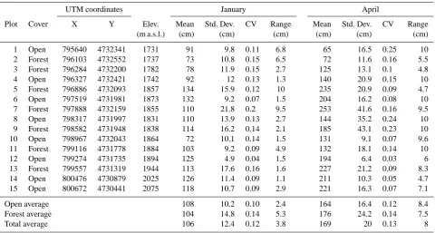
Table 1. Summary data for the study plots. Location and main statistics: mean (cm), standard deviation (cm), coefficient of variation (CV)

and semivariogram range (m).

UTM coordinates January April

Plot Cover X Y Elev. Mean Std. Dev. CV Range Mean Std. Dev. CV Range (m a.s.l.) (cm) (cm) (cm) (cm) (cm) (cm) 1 Open 795640 4732341 1731 91 9.8 0.11 6.8 65 16.5 0.25 10 2 Forest 796103 4732552 1737 73 10.8 0.15 6.5 72 11.6 0.16 5.5 3 Forest 796284 4732200 1782 78 11.9 0.15 2.7 125 13.1 0.1 4.8 4 Open 796327 4732421 1742 92 12 0.13 1.3 140 20.9 0.15 10 5 Forest 796886 4732093 1857 134 15.9 0.12 10 235 20.9 0.09 4.7 6 Open 797519 4731981 1873 132 9.2 0.07 1.5 204 16.2 0.08 10 7 Forest 797888 4732159 1855 110 21.8 0.2 9.5 253 41.6 0.16 9.5 8 Open 798317 4731997 1831 110 13.9 0.13 2.7 144 35.2 0.24 10 9 Forest 798582 4731948 1838 114 16.2 0.14 2.1 185 43.1 0.23 10 10 Open 798967 4732043 1864 72 10.1 0.14 1.5 131 9.1 0.07 9.6 11 Forest 799116 4731778 1884 103 9.2 0.09 4.9 132 18.1 0.14 10 12 Open 799274 4731735 1894 125 4.9 0.04 1.5 194 6.4 0.03 6 13 Forest 799557 4731319 1944 113 17.6 0.16 1.6 227 21.2 0.09 8.3 14 Open 800476 4730879 2025 126 11.4 0.09 1.1 211 10.3 0.05 4.7 15 Open 800672 4730441 2075 118 10.7 0.09 2.9 221 16.3 0.07 7.1 Open average 108 10.2 0.10 2.4 164 16.4 0.12 8.4 Forest average 104 14.8 0.14 5.3 176 24.2 0.14 7.5 Total average 106 12.4 0.12 3.8 169 20 0.13 8

Pyrenees, and also to represent a suitable grid size for snow depth estimations in mountain ranges worldwide. Plots were established along a transect of seven kilometers between the Hospital de Benasque and the Aigualluts sites, covering an altitudinal gradient of 340 m from 1735 to 2075 m a.s.l. (Ta-ble 1). Eight of the plots were located in forest openings where the size of the open area was less than twice the height of the surrounding trees (Pinus uncinata and silvestris of 5–15 m in height), and seven were in open areas where the size of the open area was more than five times the height of the surrounding trees. Each plot was divided into a grid of 1×1 m squares, which were sampled at each corner to yield a set of 121 data points. The average of these 121 replicates was taken to accurately represent the snow depth in the plot (ground truth).

In addition to the measurement data a synthetic data set was constructed to assess the influence of the sampling size and strategy on the estimation of the mean under controlled conditions. For the synthetic data set 5000 simulations of a random spatial field of 10×10 m were drawn for each com-bination of 10 standard deviation classes (steps of 0.025 cm from 0.025 to 0.25 cm) and four levels of spatial autocorre-lation, giving a total of 200 000 simulations. Standard devi-ation classes and levels of autocorreldevi-ation were defined ac-cording to the maximum snow depth variability and spatial autocorrelation observed in the sampled plots in the study area. Autocorrelation in the spatial fields was represented by a Gaussian semivariogram (Cressie, 1993), with the

par-tial sill parameter equal to the square of the standard devi-ation (the variance of the set) and four levels of the range parameter (from 1 m for low autocorrelation to 10 m for very high autocorrelation). The simulated spatial fields were ob-tained using the sequential Gaussian simulation algorithm, as implemented in the function predisct.gstat of the gstat pack-age (Pebesma, 2004); the R langupack-age was used for statistical analysis (R Development Core Team, 2010).

3 Statistical analysis

Snowpack variability was assessed by comparison of the dis-tribution of depths and histograms of the data. Comparison of the characteristics of the histograms derived from the data from the forest openings with those derived from the open areas could provide insights into the role of the forest canopy in snowpack variability at the plot scale.

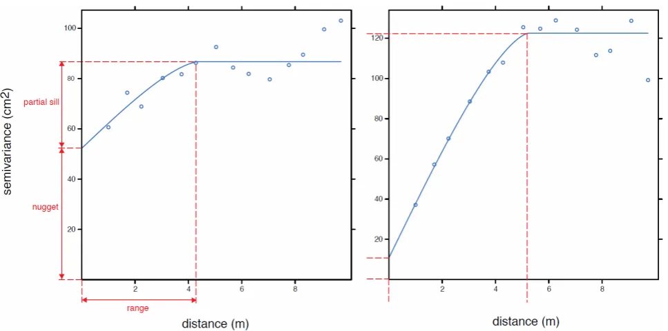
The presence of spatial correlations at the plot scale was determined for each sampling plot using a semivariogram. The semivariogram plots the average semivariance between pairs of points as a function of the distance between them. Relevant parameters of the semivariogram are the sill (the maximum value of semivariance), the nugget (the value of semivariance at the discontinuity at the origin), and the range or correlation length (the distance at which the difference in the semivariance from the sill becomes negligible). In mod-els with a fixed sill the range is the distance at which this is

(4)

620 J. I. L´opez-Moreno et al.: Variability of snow depth at the plot scale

1

2 Figure 1

3

4

Fig. 1. Illustrates semivariograms of two different empirical semivariogram (dots) and fitted circular semivariogram model (blue line) of two

sampling plots in January (left) and April (right).

first reached; for models with an asymptotic sill the range is conventionally taken to be the distance when the semi-variance first reaches 95 % of the sill (Edward et al., 1989). Here a circular semivariogram model was used. Figure 1 il-lustrates semivariograms of two different empirical semivar-iogram (dots) and fitted circular semivarsemivar-iogram model (blue line) of two sampling plots in January (left) and April (right). While the range of the autocorrelation was similar on both dates, the high nugget value of January revealed a stronger autocorrelation at short distances.

Subsets of different sample sizes (fromn=1 ton=121) were randomly extracted from each plot to assess the rela-tionship between the error of the estimate mean snow depth and the sample size. To obtain a robust estimation of SE this process was repeated 50 times for each plot using dif-ferent random subsets. The same analysis was applied to the synthetic datasets to isolate the effects of the field variance and the spatial autocorrelation on the error of the mean snow depth. Because of the large number of simulations the effect of various sampling strategies could be assessed. A sam-ple size of five replicates was used with 10 different spatial configurations and varying distances between the measure-ments, as follows: (i) random; (ii) one row at 1 m and 2 m distance; (iii) a +-shape (a central point and measurements toward the four cardinal directions) at 1, 2 and 5 m; (iv) an L-shape (northward and eastward points from a central point) at 1, 2 and 5 m; and (v) the four corners plus the central point.

4 Results

4.1 Plot scale variability

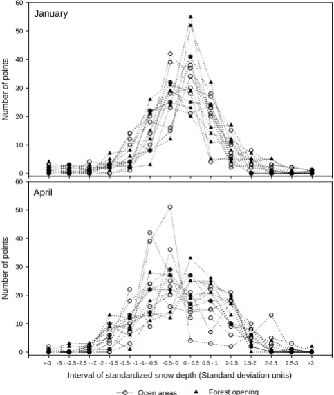
The mean, standard deviation, coefficient of variation (CV) and semivariogram range for the 15 plots are listed in Ta-ble 1; Fig. 2 shows the associated snow depth histograms. In January 2009 there was moderate variability in the snow depth among the plots, with a mean plot depth of 73–134 cm. Moreover, there was marked variability at the plot scale, with coefficients of variation ranging from 0.04 to 0.20 (mean 0.12). Despite this variability, the shape of all histograms was leptokurtic, indicating that most of the snow depths were included in only a few depth classes.

The mean snow depth among plots was more variable in April than in January, ranging from 65 to 253 cm. Snow ac-cumulation increased in most of the plots, and the increase was substantial in eight plots. Only in the two plots at the lowest altitudes (plots 1 and 2) did snow depth decrease slightly. The average within-plot variability (CV) was sim-ilar in April to that in January (mean CV = 0.12), but the range was greater, from 0.03 cm in plot 12 to 0.25 cm in plot 1. The marked leptokurtic shape of the histograms ob-served for the January data was not as evident in April. The semivariogram range varied from 1.3 to 10 m in January, and from 4.7 to 10 m in April. A range of 10 m indicates that the range over which autocorrelation is significant is greater than the maximum possible distance between points in the plots. Overall, the spatial autocorrelation was less in January (mean range = 3.8 m) than in April (mean range = 8 m). In

(5)

27

<-3 -3 - -2.5 -2.5 - -2 -2 - -1.5 -1.5- -1 -1- -0.5 -0.5- 00 - 0.5 0.5 - 1 1-1.5 1.5-2 2-2.5 2.5-3 >3 January

N

u

m

b

e

r

o

f

p

o

in

ts

0 10 20 30 40 50 60

April

Interval of standardized snow depth (Standard deviation units)

N

u

m

b

e

r

o

f

p

o

in

ts

0 10 20 30 40 50 60

Open areas Forest opening 1

2

3

Figure 2.

4

Fig. 2. Histograms of the 121 measured snow depths (standard

de-viation units) for each of the 15 plots distributed in various classes for January and April.

January the spatial autocorrelation was greater in the forest openings (mean range = 5.3 m) than in the open areas (mean range = 2.4 m). In April the spatial autocorrelation was very similar in the forest openings (mean range = 7.5 m) and the open areas (mean range = 8.4 m).

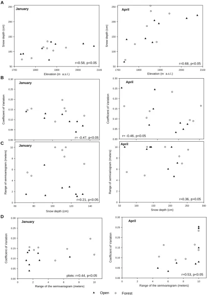
Despite the altitudinal range covered by the survey be-ing relatively low (1735 to 2075 m a.s.l.), the effect of ele-vation on the mean snow depth in both January and April (Fig. 3a) was statistically significant (p <0.05). The overall micro-scale variability of snow depth, measured by means of the CV, tended to decrease as the snowpack depth increased (Fig. 3b). The CV was statistically correlated (α <0.05) with mean snow depth, withrvalues of−0.47 and−0.46 for Jan-uary and April, respectively. The location of the plot in a forest opening or an open area appeared to be the most influ-ential factor explaining the degree of variability in January. At that time the average accumulation of snow in the forest opening plots (104 cm) was very similar to that in the open areas (108 cm), but the CV in the open areas (0.10) was lower than in forest openings (0.14). A one-way ANOVA test con-firmed that the differences in the coefficient of variation of snow depth between the two environments were statistically significant. In April, despite the CV being greater for forest openings (0.12) than open areas (0.10), the ANOVA test did not indicate a significant difference between the two

environ-ments. The semivariogram range in each plot was not related to the snow depth (Fig. 2c), but was significantly (p <0.05) positively correlated with the CV (Fig. 2d), such that the plot variability decreased the spatial autocorrelation.

4.2 Implications of sample size for snow depth estimation

A random extraction of subsets ofn=1 ton=121 samples was replicated 50 times and the means were compared with the ground truth mean (n=121). Replicates allowed for ro-bust estimation of the mean standard error and its range of variability for different sample sizes. Figure 3 shows the de-crease of the mean error, plus the 25th and 75th percentiles, as a function of the sample size from the 15 plots assessed in January and April 2009. The decrease of the mean stan-dard error expected from a purely random sample (accord-ing to the power function shown in Eq. 1) is also shown for comparison. The error decreased rapidly from small sample sizes, and the 5 % mean standard error was achieved with only four samples in each of January and April, or seven and eight samples, respectively, for a significance level of

α=0.25 (75th percentile). The observed mean error was systematically higher than obtained from the purely random sampling in January, while in April they were more similar.

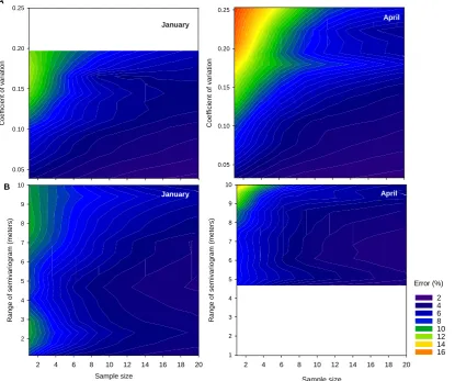
Figure 4 shows the mean, 25th and 75th percentiles of er-ror for the 15 plots. Variability amongst analyzed plots in-forms that sample size may affect in a different manner to snow depth estimation at the plot scale. Figure 4a shows the average error as a function of both the sample size and the CV. Figure 4b displays the average error as a function of the sample size and the spatial autocorrelation (the range of the correlation length) per plot. To more clearly depict patterns of change the data were smoothed using a locally weighted scatter plot smoothing-LOESS smoother (Cleveland, 1979) with one polynomial degree for a sampling proportion of 0.1. For both sampling occasions (January and April 2009) the standard error tended to be higher in plots with larger coef-ficients of variation and spatial correlation (Fig. 5a and b). In plots under the later conditions the estimate of snow depth from a single measurement could differ from the ground truth value by more than 10 % in January and 18 % in April. In these cases estimates of snow depth could contain signifi-cant errors (>10 %), even with multiple measurements. Con-versely, in those plots where snow measurements showed a low CV and low spatial autocorrelation, the standard error was notably lower than shown for the plot average in Fig. 4. Under such conditions the error could drop below 5 % with only a single measurement.

(6)

28

1

2

Elevation (m a.s.l.)

1700 1800 1900 2000 2100

S n o w d e p th ( c m ) 50 100 150 200 250 April

Elevation (m a.s.l.)

1700 1800 1900 2000 2100

S n o w d e p th ( c m ) 50 100 150 200 250 January r=0.58, p<0.05 January C o e ff ic ie n t o f V a ri a ti o n 0.00 0.05 0.10 0.15 0.20 0.25 0.30 April C o e ff ic ie n t o f V a ri a ti o n 0.00 0.05 0.10 0.15 0.20 0.25 0.30

r= -0.47, p<0.05 r= -0.46, p<0.05

January

Snow depth (cm)

60 80 100 120 140

R a n g e o f s e m iv a ri o g ra m ( m e te rs ) 0 2 4 6 8 10 April

Snow depth (cm)

50 100 150 200 250 300

R a n g e o f s e m iv a ri o g ra m ( m e te rs ) 0 2 4 6 8 10 r=0.21, p<0.05 Open Forest January

Range of the semivariogram (meters)

0 2 4 6 8 10

C o e ff ic ie n t o f V a ri a ti o n 0.00 0.05 0.10 0.15 0.20 0.25 0.30 April

Range of the semivariogram (meters)

0 2 4 6 8 10

C o e ff ic ie n t o f V a ri a ti o n 0.00 0.05 0.10 0.15 0.20 0.25 0.30

plots: r=0.44, p<0.05 r=0.53, p<0.05

r=0.68, p<0.05 r=0.36, p>0.05 A B C D

3 Figure 3.

4

Fig. 3. Relationships between (A) snow depth and altitude, (B) snow depth and coefficient of variation, (C) snow depth and semivariogram

range, and (D) coefficient of variation and semivariogram range.

(7)

29

1

2

3

Sample size

0 5 10 15 20 25 30 35 40

E

rr

o

r

(%

)

0 2 4 6 8 10 12 14

Sample size

0 5 10 15 20 25 30 35 40

Mean Error 25th percentile 75th percentile Error calculated according to power law a. January b. April

4 Figure 4

5

Fig. 4. Decrease in snow depth estimation error at the plot scale for various sample sizes. The thick line is the average error, and the thin

lines are the 25th and 75th percentiles obtained from 50 replications. The grey dashed line is the error calculated according to a power law.

30

1

C

o

e

ff

ic

ie

n

t

o

f

v

a

ri

a

ti

o

n

0.05 0.10 0.15 0.20 0.25

Sample size

2 4 6 8 10 12 14 16 18 20

R

a

n

g

e

o

f

s

e

mi

v

a

ri

o

g

ra

m

(

me

te

rs

)

1 2 3 4 5 6 7 8 9 10

2 4 6 8 10 12 14 16 Error (%)

Co

e

ff

ic

ie

n

t

o

f

v

a

ri

a

ti

o

n

0.05 0.10 0.15 0.20 0.25

April

April January

Sample size

2 4 6 8 10 12 14 16 18 20

Ra

n

g

e

o

f

s

e

mi

v

a

ri

o

g

ra

m

(

me

te

rs

)

2 3 4 5 6 7 8 9 10

January A

B

2

3 Figure 5.

4

Fig. 5. Average error for various sample sizes according to (A) the coefficient of variation and (B) the spatial autocorrelation. The white

areas correspond to ranges of the y-axis without data in one of the surveys.

(8)

31

1

2

3

Range = 1 meter

S

ta

n

d

a

rd

d

e

v

ia

ti

o

n

(

c

m

)

0.04 0.06 0.08 0.10 0.12 0.14 0.16 0.18

Sample size

2 4 6 8 10 12 14 16 18

S

ta

n

d

a

rd

d

e

v

ia

ti

o

n

(

c

m

)

0.04 0.06 0.08 0.10 0.12 0.14 0.16 0.18

2 4 6 8 10 12 14 16 18

Sample size

0 3 6 9 12 15 18 Error (%) Range = 1 meters Range = 4 meters

Range = 7 meters Range = 10 meters 5

5 5

10 10

5 5

5

10 10

5 5

5

10 10

5 5

5

10 10

4 Figure 6.

5

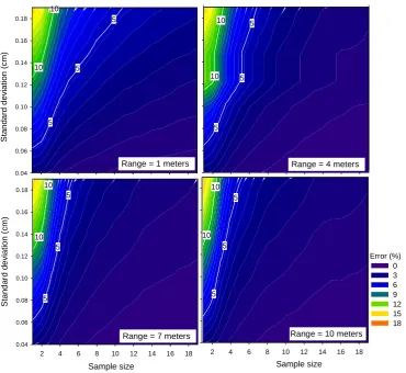
Fig. 6. Average error for various sample sizes derived from simulated plots according to various standard deviation levels and 4 classes of

spatial autocorrelation.

4.3 Effect of coefficient of variation, spatial autocorrelation and sampling strategy on snow depth estimation

In natural situations completely random sampling of snow is rarely achievable because of a variety of difficulties includ-ing terrain complexity. Thus, in most real-world studies a specific sampling strategy is used, such as taking a number of samples in a line, plus or an L. It is plausible that a par-ticular sampling strategy is better able to capture the spatial variability in an autocorrelated field. To assess this possibil-ity we simulated 200 000 plots composed of 121 points with an equal average snow depth (100 cm), but with differing lev-els of standard deviation and spatial autocorrelation.

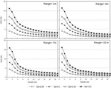
The mean standard error for various levels of standard de-viation and spatial autocorrelation for the random sampling is shown in Fig. 6. Figure 7 shows the example of four levels of standard deviation for various levels of spatial autocorrela-tion. Both figures (Figs. 6 and 7) demonstrate that variability in snow depth at the plot scale (measured by the standard de-viation) explained the different degrees of accuracy relative to the ground truth data. Thus, the 4 degrees of spatial

auto-correlation provided almost identical patterns of a decrease in error as sample size increased and standard deviation de-creased. Variability in the decrease in mean standard error with sample size depended largely on the standard deviation of the spatial field, while the extent of spatial correlation was far less important. However, differences were also found for varying levels of spatial autocorrelation, and the mean standard error was slightly lower in cases with higher auto-correlation because of their implicit lower spatial variability. When the standard deviation exceeded 0.1 cm a single mea-surement provided a mean error>10 %, and the error ap-proached 20 % when the standard deviation was 0.2 cm. The decrease in error according to sample size approximated the theoretical exponential decay for a purely random variable. From Fig. 7 it can be seen that 4 measurements per plot re-sulted in errors<5 % if the standard deviation was<0.1 cm. Five measurements were needed to achieve a similar accu-racy with a standard deviation of 0.15 cm, while seven or eight measurements were needed for a standard deviation of 0.2 cm. Five measurements provided error estimates<10 % for all degrees of spatial autocorrelation tested.

(9)

32

Range= 1m

E

rr

o

r

(%

)

0 5 10 15 20

Sample size

0 2 4 6 8 10 12 14 16 18

E

rr

o

r

(%

)

0 5 10 15 20

Sample size

0 2 4 6 8 10 12 14 16 18 Range= 4m

Range= 10 m Range= 7m

Sd=0.05 Sd=0.1 Sd=0.15 Sd= 0.2

1 Figure 7

2

Fig. 7. Examples showing the decrease in average error according to sample size for 4 standard deviation levels with various classes of

spatial autocorrelation.

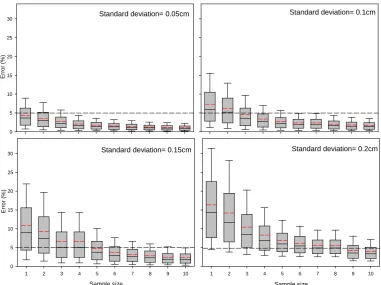
Figure 8 shows the variability of the mean standard error amongst the 5000 simulations for different sample sizes at four levels of standard deviation (0.05, 0.1, 0.15 and 0.2 cm) and the same level of spatial autocorrelation (semivariogram range = 4 m). The average values shown in Figs. 6 and 7 can mask substantial variability (Fig. 8), and even with a low standard deviation (i.e. 0.05 or 0.1 cm) inaccurate snow depth estimates are possible if the sample size is<4 measurements. In the case of plots with large snow depth variability, a small number of measurements may lead to marked deviation from the ground truth mean. Thus, there was a 25 % probability of an error approaching 10 % if less than five measurements were used when the standard deviation exceeded 0.1 cm. In general, Fig. 8 suggests that a single measurement is highly unreliable as an estimate of snow pack depth at the plot scale. There was 10 % probability of an error of 9, 16, 23 and 32 % for standard of 0.05, 0.1, 0.15 and 0.2 cm, respectively.

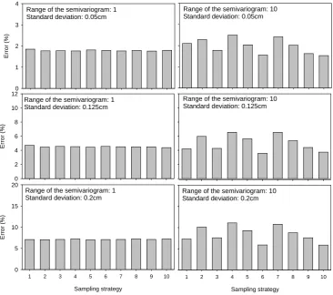
Snow depth estimates from 5 measurements using 10 dif-ferent configurations of shape (row, L-shape, +-shape and random) and distance between measurements (1, 2 and 5 m) were compared with the ground truth mean. In Fig. 9 each panel represents a given combination of three standard de-viations (0.05, 0.125 and 0.2 cm) and 2 levels of spatial au-tocorrelation (semivariogram range = 1 and 10 m). With no spatial autocorrelation the sampling strategy did not impact on the snow depth estimate. However, with a high spatial

au-tocorrelation a smaller error was obtained when the distance between measurements was greater, as shown with sampling at the center and the four corners of the plot 5 m away, in a “+” shape (configurations 10 and 6 in Fig. 9). For all three spatial configurations (line, “+” or “L” shapes) the largest er-rors were obtained when the distance between measurements was only 1 m. Random sampling and a 2 m spacing provided intermediate levels of accuracy, with the measurements along a line being slightly more accurate than the “+” or “L” con-figurations. Under high snow variability condition (sd = 0.2), the results indicate that a 5 m spacing of measurements could result in an improvement in mean snow depth estimates of approximately 5 % relative to a spacing of 1 m, while chang-ing the spacchang-ing from 1 to 2 m could increase accuracy up to 3 %.

5 Discussion

The data from two snow surveys (January and April 2009) carried out in the Pyrenees (Spain) showed that there was marked variability in the snowpack depth within each of the 10×10 m study plots. Such heterogeneity can prevent accu-rate estimates of snow depth being obtained. To improve the accuracy of snowpack estimates, it is necessary to average several measurements taken within each plot.

(10)

33

1

E

rr

o

r

(%

)

0 5 10 15 20 25

30 Standard deviation= 0.05cm

Standard deviation= 0.1cm

Sample size

1 2 3 4 5 6 7 8 9 10

E

rr

o

r

(%

)

0 5 10 15 20 25 30

Sample size

1 2 3 4 5 6 7 8 9 10

Standard deviation= 0.15cm Standard deviation= 0.2cm

2 Figure 8

3

4

Fig. 8. Variability in error estimates among the 5000 simulations involving various sample sizes and 4 levels of standard deviation. The solid

lines indicate the average, the dashed lines indicate the mean, the boxes indicate the 25th and 75th percentiles, and the bars indicate the 10th and 90th percentiles.

The two surveys undertaken in the present study were not sufficient to provide evidence of seasonal patterns, but dif-ferences between the two sampling periods were observed. It has been found that within a few months snow density and temperature can change markedly (Fassnacht et al., 2010), and similar variability was found in this study with respect to snow depth variability at the plot scale, the spatial autocorre-lation of snow depth, and the role of the forest canopy. All these factors can affect the minimum sample size and/or the sampling strategy necessary to satisfactorily represent snow depth at the plot scale.

Previous studies have identified large spatial variability at the plot scale (Tarboton et al., 2000; Pomeroy et al., 2001; Anderton et al., 2002), which is a consequence of the par-ticular characteristics of the terrain, the amount of accumu-lated snow, and the influence of surrounding forest. The presence and quantity of boulders, branches and irregular-ities in the terrain clearly influenced the variability among the plots in the study area. For each of the surveys a statis-tically significant correlation was found between the mean snow depth and the variability in each plot. An explana-tion for this relaexplana-tionship is that irregularities in the terrain are constant in size, and thus their relative influence on the snow depth decreases as the snowpack depth increases (Fass-nacht and Deems, 2006; L´opez-Moreno and Latron, 2008).

In both surveys higher snow depth variability was found in the plots located in forest openings relative to those in open areas. This can be explained in part by the horizontal and vertical structure of trees within forest stands, local shadow effects (Musselman et al., 2008) and the emission of long-wave radiation from surrounding trees, differential ablation rates as consequence of litter on the snow, and the increased probability of the presence of tree branches and/or stumps on the ground (Pomeroy et al., 2001; St¨ahli et al., 2009). However, certain plots in open areas exhibited the greatest variability among all plots in April 2009; these plots were lo-cated at the lowest altitudes, where the snowpack was thinner and local topography had a greater influence.

Semivariograms have been used to detect significant spa-tial autocorrelation (Essery et al., 1999; Deems et al., 2006; Jost et al., 2007; Kronholm and Birkeland, 2007), but in most cases have been used at the slope scale. Watson et al. (2006) and Jost et al. (2007) assumed variability at the plot scale to be random, and analyzed variability at the watershed-scale from stratified data, using multiple replicates at the plot scale to conduct geostatistical analyses to assess local variability. In this study we found that spatial autocorrelation occurred at the plot scale, but varied markedly among plots and tended to be greater in the forest openings. This is probably because of a spatial trend in forest canopy processes affecting the energy

(11)

34

1

E

rr

o

r

(%

)

0 1 2 3 4

E

rr

o

r

(%

)

0 2 4 6 8 10 12

Sampling strategy

1 2 3 4 5 6 7 8 9 10

E

rr

o

r

(%

)

0 5 10 15 20

Sampling strategy

1 2 3 4 5 6 7 8 9 10

1: Random; 2: Row 1m; 3: Row 2m; 4: Plus 1m; 5: Plus 2m; 6: Plus 5m 7: L 1m; 8: L 2m; 9: L 5m; 10: center and four corners

Range of the semivariogram: 1 Standard deviation: 0.05cm

2 Figure 9

3

Fig. 9. Impact of sampling strategy on error estimation at the plot scale.

balance and wind redistribution, including shadow and wind shield effects, and the emission of long-wave radiation. As in this study, Holmgren et al. (1998) recognized the existence of well-defined sills for the residual spatial variances at a range of about 10 m. For an area with a sparse canopy, Deems et al. (2006) showed that the correlation length was a function of canopy structure and terrain, and was in the order of 15 to 20 m. However, using spectral analysis Trujillo et al. (2007) did not find a clear relationship between topographic relief and the correlation length. For the same study sites the spa-tial memory of snow depth in the forested areas was similar to the vegetation height field, and increased in open areas as a consequence of wind redistribution (Trujillo et al., 2009). Moreover, it is logical to assume that the range actually be much greater if a slightly larger plot overlapped both vege-tated and open areas. This is a particularly relevant question as the considered plot is of larger size than considered in this study.

To obtain reliable snow depth estimates at a 10×10 m plot scale it is necessary to make multiple measurements. With a single measurement the estimation of snow depth in the plot is likely to be highly biased. The deviation from the ground

truth mean with different sample sizes was mostly associ-ated with snow depth variability at the plot scale. From the data obtained it was possible to infer a relationship between the degree of spatial autocorrelation and the mean standard error. However, this may have been a consequence of the relationship in this data set between the CV and the semivar-iogram range. A sensitivity analysis conducted with multiple simulations of snow depth for various autocorrelation ranges showed that the effect of autocorrelation on estimates of the mean was much lower than the standard deviation of the field. However, in the presence of spatial autocorrelation the sampling strategy became a relevant factor; snow depth esti-mates improved by maximizing the distance between sam-pling points within the plot and increasing the number of measurements. Specific configurations of the snow measure-ments did not make a significant difference to the quality of the estimates. Overall our results suggest that snow sampling should prioritize the collection at least five snow depth mea-surements at a minimum 2 m spacing to represent a 10×10 m plot sized area. The specific numbers presented here relating sample size and snow depth estimates are closely related to the topographic and climatic characteristics of the study area,

(12)

628 J. I. L´opez-Moreno et al.: Variability of snow depth at the plot scale and the specific plot size considered in this study. The aim

of this research was not to provide guidance for sampling in other geographical areas or surface terrain characteristics, but highlights the usefulness of considering this type of analysis during the planning of snow surveys. Initial measurements of numerous snow depths at the plot scale can be used to de-termine the measurement variability of a location, and can help to decide how many samples should be taken to repre-sent each survey point. This approach should improve the representativeness of the dataset. A better understanding of the factors that influence the spatial and temporal patterns of snowpack variability and spatial autocorrelation at the plot scale will aid efforts to obtain high quality snow datasets. We have presented information of 15 plots in two different periods of the year. However, we could find a larger range of variability and spatial correlation if a more detailed tem-poral resolution of the surveys, and a higher variety of envi-ronments (i.e. sub-canopy plots, high mountain areas, etc.) would have been sampled. Further research could be ad-dressed to analyze the dynamic nature of the variability (in space and time), which could reveal additional information for improving the accuracy of snow depth estimation.

6 Conclusions

Based on a 1 m sampling resolution, snow depth exhibited marked variability at a 10×10 m plot scale, especially in forest openings. This variability explains the need to aver-age several measurements in each plot to obtain a reliable estimate of the snow depth. The number of measurements needed depends on the degree of variability of the snowpack at the plot scale, and the desired accuracy. In this study five measurements produced an error of<10 % even under high variability conditions. With high micro-scale variabil-ity the collection of 8 measurements reduced the error to 5 % in more than 75 % of cases. Snow depth variability is often spatially autocorrelated. With no spatial autocorrelation the sampling strategy did not impact on the snow depth estimate. However, with a high spatial autocorrelation a smaller error was obtained when the distance between measurements was greater. In such cases spacing the measurements within the plot independently of the spatial configuration enhanced the accuracy of the snow depth estimates. Thus, under high spa-tial autocorrelation (semivariogram range = 10 m) and high snow variability condition (sd = 0.2 cm), the results indicate that a 5 m spacing of measurements could result in an im-provement in mean snow depth estimates of approximately 5 % relative to a spacing of 1 m, while changing the spacing from 1 to 2 m could increase accuracy up to 3 %.

Acknowledgements. This work was supported by research projects

CGL2006-11619/HID and CGL2011-27536 (Hidrologia nival en el pirineo central espa˜nol: variabilidad espacial, importancia hidrologica y su respuesta a la variabilidad y cambio clim´atico), financed by the Spanish Commission of Science and Technology

and FEDER, ACQWA (FP7-ENV-2008-1-212250) and the projects “La nieve en el Pirineo aragonés: Distribución especial y su respuesta a las condiciones climáticas”, financed by “Obra Social La Caixa” and “Influencia del cambio climático en el turismo de nieve-CTTP1/10”, financed by the Comisión de Trabajo de los Pirineos, CTP. Data collection was assisted by Gonzalo López, Pablo Corella and Mario Morellón; their efforts are acknowledged with thanks.

Edited by: S. Dery

References

Anderton, S. P., White S. M., and Alvera, B.: Micro-scale spatial variability and the timing of snow melt runoff in a high mountain catchment, J. Hydrol., 268, 158–176, 2002.

Cleveland, W. S.: Robust Locally Weighted Regression and Smoothing Scatterplots, J. Am. Stat. Assoc., 74(368), 829–836, 1979.

Cline, D., Elder, K., and Bales, R.: Scale Effects in a Distributed Snow Water Equivalence and Snowmelt Model for Mountain Basins, Hydrol. Process., 12, 1527–1536, 1998.

Cressie, N. A. C.: Statistics for Spatial Data, Wiley, New York, 900 pp., 1993.

Deems, J. S., Fassnacht, S. R., and Elder, K. J.: Fractal distribution of snow depth from LiDAR data, J. Hydrometeorol., 7(2), 285– 297, 2006.

Dressler, K. A., Fassnacht, S. R., and Bales, R. C.: Comparison of snow telemetry (SNOTEL) and snowcourse measurements in the Colorado River Basin, J. Hydrometeorol., 7(4), 705–712, 2006. Edward, H., Isaaks, E. H., and Srivastava, R. M.: An introduction

to applied geostatistics, Oxford University Press, Oxford (UK), 561 pp., 1989.

Elder, K., Rosenthal, W., and Davis, R. E.: Estimating the spatial distribution of snow water equivalence in a montane watershed, Hydrol. Process., 12, 1793–1808, 1998.

Erickson, T. A., Williams, M., and Winstral, A.: Persistence of to-pographic controls on the spatial distribution of snow in rugged mountain terrain, Colorado, United States, Water Resour. Res., 41, W04014, doi:10D1029/2003WR002973, 2005.

Erxleben, J., Elder, K., and Davis, R.: Comparison of spatial in-terpolation methods for estimating snow distribution in the Col-orado Rocky Mountains, Hydrol. Process., 16, 3627–3649, 2002. Essery, R., Li, L., and Pomeroy, J. W: A distributed model of blow-ing snow over complex terrain, Hydrol. Process., 13, 2423–2438, 1999.

Fassnacht, S. R. and Deems, J. S.: Measurement sampling and scal-ing for deep montane snow depth data, Hydrol. Process., 20(4), 829–838, 2006.

Fassnacht, S. R., Dressler, K. A., and Bales, R. C.: Snow water equivalent interpolation for the Colorado River Basin from snow telemetry (SNOTEL) data, Water Resour. Res., 39(8), W1208, doi:10.1029/2002WR001512, 2003.

Fassnacht, S. R., Heun, C. M., López-Moreno, J. I., and Latron, J.: Variability of snow density measurements in the Esera val-ley, Pyrenees mountains, Spain, Cuadernos de Investigación Ge-ográfica, 36(1), 59–72, 2010.

Haefner, H., Seidel, K., and Releer, S.: Applications of snow cover mapping in high mountain regions, Phys. Chem. Earth, 22(3–4),

(13)

275–278, 1997.

Holmgren, J., Sturm, M., Yankielun, N. E., and Koh, G.: Extensive measurements of snow depth using FM-CW radar, Cold Reg. Sci. Technol., 27, 17–30, 1998.

Jost, G., Weiler, M., Gluns, D. R., and Alila, Y.: The influence of forest and topography on snow accumulation and melt at the watershed-scale, J. Hydrol., 347, 101–115, 2007.

Kronholm, K. and Birkeland, K. W.: Reliability of sampling designs for spatial snow surveys, Comput. Geosci., 33(9), 1097–1110, 2007.

L´opez-Moreno, J. I. and Latron, J.: Influence of forest canopy on snow distribution in a temperate mountain range, Hydrol. Pro-cess., 22(1), 117–126, 2008.

L´opez-Moreno, J. I. and Nogu´es-Bravo, D.: Interpolating snow depth data: a comparison of methods, Hydrol. Process., 20(10), 2217–232, 2006.

L´opez-Moreno, J. I., Vicente-Serrano, S. M., and Lanjeri, E.: Map-ping of snowpack distribution over large areas using GIS and interpolation techniques, Clim. Res., 33, 257–270, 2007. Molotch, N. P. and Bales, R. C.: Scaling snow observations

from the point to the grid element: implications for ob-servation network design, Water Resour. Res., 41, W11421, doi:10.1029/2005WR004522, 2005.

Musselman, K. N., Molotch, N. P., and Brooks, P. D.: Quantifying the effects of forest vegetation on snow accumulation, ablation and potential meltwater inputs, Valles Caldera National Preserve, NM, USA, Hydrol. Process., 22, 2767–2776, 2008.

Neumann, N. N., Derksen, C., Smith, C., and Goodison, B.: Char-acterizing local scale snow cover using point measurements dur-ing the winter season, Atmos. Ocean, 44(3), 257–269, 2006. Nielsen, D. R. and Wendroth, O.: Spatial and temporal statistics.

Sampling field soils and vegetation, Geoecology, Reiskirchen (Germany), 398 pp., 2003.

Pebesma, E. J.: Multivariable geostatistics in S: the gstat package, Comput. Geosci., 30, 683–691, 2004.

Pomeroy, J. W., Hanson, S., and Faria, D.: Small scale variation in snowmelt energy in a boreal forest: an additional factor control-ling depletion of snow cover?, in: Proceedings of 58th Eastern Snow Conference, Ottawa, Ontario, Canada, May 2001. Rovansek, R. J., Kane, D. L., and Hinzman, L. D.: Improving

esti-mates of snowpack water equivalent using double sampling, 50th Eastern Snow Conference, 157–163, 1993.

R Development Core Team: R: A Language and Environment for Statistical Computing, R Foundation for Statistical Computing, Vienna, Austria, ISBN 3-900051-07-0, http://www.R-project. org, 2010.

St¨ahli, M., Jonas, T., and Gustafsson, D.: The role of snow intercep-tion in winter-time radiaintercep-tion processes of a coniferous sub-alpine forest, Hydrol. Process., 23, 2498–2512, 2009.

Tarboton, D., Blösch, G., Cooley, K., Kirnbauer, R., and Luce, C.: Spatial snow cover processes at Kühati and Reynold Creek, in: Spatial Patterns in Catchment Hydrology, edited by: Grayson, R. and Blösch, G., Cambridge University Press, Cambridge, UK, 158–186, 2000.

Trujillo, E., Ram´ırez, J. A., and Elder, K. J.: Topographic, meteo-rologic, and canopy controls on the scaling characteristics of the spatial distribution of snow depth fields, Water Resour. Res., 43, W07409, doi:10D1029/2006WR005317, 2007.

Trujillo, E., Ram´ırez, J. A., and Elder, K. J.: Scaling properties and spatial organization of snow depth fields in sub-alpine forest and alpine tundra, Hydrol. Process., 23(11), 1575–1590, 2009. Watson, F. G. R., Anderson, T. N., Newman, W. B., Alexander,

S. E., and Garrot, R. A.: Optimal sampling techniques for esti-mating mean snow water equivalents in stratified heterogeneous landscapes, J. Hydrol., 328, 432–452, 2006.