Multi-Step Preconditioned Newton Methods for
Solving Systems of Nonlinear Equations
Fayyaz Ahmad1,2,3,*, Malik Zaka Ullah1,4, Ali Saleh Alshomrani4, Shamshad Ahmad5, Aisha M. Alqahtani6and L. Alzaben4
1 Dipartimento di Scienza e Alta Tecnologia, Universita dell’Insubria, Via Valleggio 11, Como 22100, Italy;
2 Departament de Física i Enginyeria Nuclear, Universitat Politècnica de Catalunya, Eduard Maristanu 10,
Barcelona 08019, Spain
3 UCERD (Pvt) Ltd, Islamabad, Pakistan
4 Department of Mathematics, King Abdulaziz University, Jeddah 21589, Saudi Arabia;
[email protected] (A.S.A.); [email protected] (L.A.)
5 Heat and Mass Transfer Technological Center, Technical University of Catalonia, Colom 11, Terrassa 08222,
Spain; [email protected]
6 Princess Nourah bint Abdulrahman University Riyadh, Saudi Arabia; [email protected]
* Correspondence: [email protected]; Tel.: +34-63-206-6627
Abstract: The study of different forms of preconditioners for solving a system of nonlinear equations, by using Newton’s method, is presented. The preconditioners provide numerical stability and rapid convergence with reasonable computation cost, whenever chosen accurately. Different families of iterative methods can be constructed by using a different kind of preconditioners. The multi-step iterative method consists of a base method and multi-step part. The convergence order of base method is quadratic and each multi-step add an additive factor of one in the previously achieved convergence order. Hence the convergence of order of anm-step iterative method ism+1. Numerical simulations confirm the claimed convergence order by calculating the computational order of convergence. Finally, the numerical results clearly show the benefit of preconditioning for solving system of nonlinear equations.
Keywords:systems of nonlinear equations; nonlinear preconditioners; multi-step iterative methods; Frozen Jacobian
When computing simple roots of a system of nonlinear equations, Newton’s method [1–4] is a classical, well studied procedure that offers quadratic convergence, under suitably mild regularity assumptions. Many researchers have proposed higher order efficient iterative method [5–12] for solving system of nonlinear equations. Recently, some authors have constructed multi-step iterative methods [13–15] for solving system of nonlinear equations. The main benefit of multi-step iterative methods is hidden in the multi-step part. Because, the Jacobian factorization information from the base method is utilized in the multi-step part repeatedly to enhance the convergence order at the cost of the solution of lower and upper triangular systems and a single evaluation of the system of nonlinear equations. X. Wu [16] wrote a note on the improvement of Newton’s method for systems of nonlinear equations. In his note, the author introduced the idea of nonlinear preconditioners and showed that the improved Newton method enjoyed the quadratic convergence. Jose et al. [17] used the idea of nonlinear preconditioning to improve the Newton method, for solving the system of nonlinear equations with known multiplicities. Aslam et al. [18] proposed iterative methods for solving nonlinear equations with unknown multiplicity with the help of nonlinear preconditioners. In the another article Aslam and his co-researcher [19] proposed a preconditioned double Newton method with quartic convergence order for the solving system of nonlinear equations. What they have proposed is the following. Let
be the system of nonlinear equations and let us suppose that only simple roots are present. Here
x = [x1,x2,· · ·,xn]T. Assume G(x) = [g1(x),g2(x),· · ·,gn(x)]T is a function which is non-zero
everywhere in its definition domain. We define a new function
Q(x) =G(x)F(x) = [[G(x)]]F(x) = [[F(x)]]G(x), (2)
whereis the element-wise multiplication and[[·]]represent the diagonal matrix, having as main diagonal its argument. The first order Fréchet derivative of (2) can be computed as
Q0(x) = [[F(x)]]G0(x) + [[G(x)]]F0(x)
= [[G(x)]]F0(x) + [[F(x)]] [[G(x)]]−1G0(x). (3)
The application of Newton method to (2) gives
xk+1=xk−Q0(xk)−1Q(xk) =xk−
F0(x) + [[F(x)]] [[G(x)]]−1G0(x)−1F(x). (4)
The convergence order of (4) is quadratic, because the considered scheme is the Newton method for solving the preconditioned system of nonlinear equationsQ(x) =0. If we takeG(x) =exp(βββx)
then (4) can be written as
xk+1=xk− F0(x) + [[βββF(x)]]−1F(x), (5)
whereβββ= [β1,β2,· · ·,βn]T.
1. Our proposal
In this section, we develop some preconditioned iterative methods for solving systems of nonlinear equations. We generalize the idea of preconditioning in such a way that the quadratic convergence will be guaranteed, under the usual regularity requirements. If we replaceG(x)byexp(G(x))in (4), then we obtain
xk+1=xk−
F0(xk) + [[F(xk)]]G0(xk)
−1
F(xk). (6)
Notice thatG0(x)is a matrix that could be a diagonal matrix, but also a generic dense matrix. We proposed the following generalization of (6)
xk+1=xk−
F0(xk) +M1(xk) [[F(xk)]]M2(xk)
−1
F(xk), (7)
whereM1(x)andM2(x)are matrices of sizen. In the next development, we see that[[F(x)]]is not the
only option. Letp(x)be a scalar function and let us define the following preconditioned system of nonlinear equations
Q(x) =p(x)F(x) = [p(x)f1(x),p(x)f2(x),· · ·,p(x)fn(x)]T. (8)
The first order Fréchet derivative of (8) can be computed as
Q0(x) =p(x)F0(x) +F(x)∇p(x)T Q0(x) =p(x)
F0(x) +F(x)
∇
p(x)T p(x)
where p(x)F0(x)means the element-wise product of p(x)with each element ofF0(x)and / in
∇p(x)T
p(x)
is element-wise division. The application of the Newton method to (8) gives
xk+1=xk−
F0(xk) +F(xk)
∇
p(xk)T p(xk)
−1
F(xk). (10)
Again, if we replacep(xk)byexp(p(xk))in (10), then we have
xk+1=xk−
F0(xk) +F(xk)∇p(xk)T
−1
F(xk). (11)
The following generalization of (11) can be obtained
xk+1=xk−
F0(xk) +F(xk)V(xk)T
−1
F(xk) and (12)
xk+1=xk−
F0(xk) +V(xk)F(xk)T
−1
F(xk), (13)
whereV(xk) = [v1(xk),v2(xk),· · ·,vn(xk)]T. Other possibilities could be
xk+1=xk−
F0(xk) +M1(xk)F(xk)V(xk)TM2(xk)
−1
F(xk) and (14)
xk+1=xk−
F0(xk) +M1(xk)V(xk)F(xk)TM2(xk)
−1
F(xk). (15)
Further, we write the multi-step version of the proposed generalizations
Base method−→
x0=initial guess
Aφφφ1=F(x0)
x1=x0−φφφ1
Multi-step part→
for j=2,m Aφφφj =F xj−1
xj=xj−1−φφφj end
x0=xm,
(16) where A= Iterative method
F0(x) +M1(x) [[F(x)]]M2(x) (7)
F0(x) +F(x)V(x)T (12) F0(x) +V(x)F(x)T (13) F0(x) +M1(x)F(x)V(x)TM2(x) (14)
F0(x) +M1(x)V(x)F(x)TM2(x) (15)
The famous Newton multi-step iterative method can be written as
Base method−→
x0=initial guess
F0(x0)φφφ1=F(x0)
x1=x0−φφφ1
Multi-step part→
for j=2,m
F0(x0)φφφj =F xj−1
xj=xj−1−φφφj end
x0=xm.
(17)
2. Convergence Analysis
In this section we gice in detail the proofs of convergence order of (16) only form=2, while for the casem≥3 we use mathematical induction.
Theorem 2.1. LetF:Γ ⊆Rn →
Rn be sufficiently Frechet differentiable on an open convex neighborhood
Γofx∗ ∈ Rn withF(x∗) = 0, det(F0(x∗)) 6= 0, and with well defined quantities||M
1(xk)||,||M2(xk)||,
||V(xk)||. Then the sequence{xk}generated by (16) converges tox∗with local order of convergence at least three for m=2. Furthermore, the following error inequality
||ek+1|| ≤ ||L|| ||ek||3 (18)
is satisfied, whereek =xxxk−x∗,ekp=
p times
z }| {
(ek,ek,· · ·,ek),ek= [(ek)1,(ek)2,· · ·,(ek)n]Tand
||L||=
Iterative method
2||C2||2+3||C2|| ||M1(x0)|| ||M2(x0)||+ (||M1(x0)|| ||M2(x0)||)2
||e0||3 (7)
2||C2||2+3||C2|| ||V(x0)||+||V(x0)||2
||e0||3 (12)
2||C2||2+3||C2|| ||V(x0)||+||V(x0)||2||e0||3 (13)
2||C2||2+3||C2|| ||M1(x0)|| ||M2(x0)|| ||V(x0)||+ (||M1(x0)|| ||M2(x0)|| ||V(x0)||)2
||e0||3 (14)
2||C2||2+3||C2|| ||M1(x0)|| ||M2(x0)|| ||V(x0)||+ (||M1(x0)|| ||M2(x0)|| ||V(x0)||)2
||e0||3 (15)
. (19)
Proof. TheqthFrechet derivative ofFatv∈Rn,q≥1, is theq−linearfunctionF(q)(v):
q times
z }| {
RnRn· · ·Rn
such thatF(q)(v) u1,u2,· · ·,uq ∈ Rn. The Taylor’s series expansion ofF(x0)aroundx∗ can be
written as
F(x0) =F(x∗+x0−x∗) =F(x∗+e0), =F(x∗) +F0(x∗)e0+ 1
2!F
00
(x∗)e02+ 1
3!F
(3)(x∗
)e03+· · ·,
=F0(x∗)
e0+ 1
2!F
0(x∗)−1
F00(x∗)e02+ 1
3!F
0(x∗)−1
F(3)(x∗)e03+· · ·
,
=C1
e0+C2e02+C3e03+O
e04
, (20)
whereC1=F0(x∗)andCs = s1!F
0(x∗)−1
F(s)(x∗)fors≥2. From (20), we can calculate the Fréchet derivative ofFas
F0(x0) =C1
I+2C2e0+3C3e02+4C3e03+O
e04
whereIis the identity matrix. Before to proceed further, first we compute the norm bounds for
B(x)∈nM1(x) [[F(x)]]M2(x),F(x)V(x)T,V(x)F(x)T,M1(x)F(x)V(x)TM2(x),M1(x)V(x)F(x)TM2(x)
o
.
B(x0) =M1(x0) [[F(x0)]]M2(x0) =M1(x0) [[C1
e0+C2e20+O
e30
]]M2(x0) ||B(x0)|| ≤ ||C1|| ||M1(x0)|| ||M2(x0)|| ||e0||
(22)
B(x0) =F(x0)V(x0)T =C1
e0+C2e20+O
e30
V(x0)T ||B(x0)|| ≤ ||C1|| ||V(x0)|| ||e0||
(23)
B(x0) =V(x0)F(x0)T =V(x0)
C1
e0+C2e20+O
e30T
||B(x0)|| ≤ ||C1|| ||V(x0)|| ||e0||
(24)
B(x0) =M1(x0)F(x0)V(x0)TM2(x0) =M1(x0)
C1
e0+C2e20+O
e30
V(x0)T M2(x0) ||B(x0)|| ≤ ||C1|| ||M1(x0)|| ||M2(x0)|| ||V(x0)|| ||e0||
(25)
Notice that all the expressions forB(x)are of ordereand this is essential in proving the quadratic convergence.
B(x0) =M1(x0)V(x0)F(x0)TM2(x0) =M1(x0)V(x0)
C1
e0+C2e20+O
e30TM2(x0) ||B(x0)|| ≤ ||C1|| ||M1(x0)|| ||M2(x0)|| ||V(x0)|| ||e0||
(26)
A=F0(x0) +B(x0) =C1
I+2C2e0+C−11B(x0) +O(e20)
A−1=I−2C2e0−C−11B(x0) +O((e0)i1(e0)i2)
C−11
(27)
The explanation to use the notationO((e0)i1(e0)i2)is that the quadratic terms are not of the forme
2 0
because ofB(x0). By using (27), we deduce
A−1F(x0) =
I−2C2e0−C−11B(x0) +O((e0)i1(e0)i2)
C1−1C1
e0+C2e20+O
e30
=e0+C2e20−2C2e02−C−11B(x0)e0+O
(e0)i1(e0)i2(e0)i3
e1=e0−e0+C2e20+C−11B(x0)e0+O
(e0)i1(e0)i2(e0)i3
e1=C2e20+C1−1B(x0)e0+O
(e0)i1(e0)i2(e0)i3
The error equatione1tells that the order of convergence of base method of (16) is quadratic because
C−11B(x0)e0is a second order term ine0. By using (28), (22), (23), (24), (25) and (26) , we get
F(x1) =C1
e1+O
e21 =C1
C2e20+C1−1B(x0)e0+O
(e0)i1(e0)i2(e0)i3
e2=e1−A−1F(x1) =C2e20+C1−1B(x0)e0−
I−2C2e0−C−11B(x0) +O((e0)i1(e0)i2)
C2e20+C1−1B(x0)e0
+O(e0)i1(e0)i2(e0)i3(e0)i4
=2C22e30+2C2e0C1−1B(x0)e0+C1−1B(x0)C2e20+C−11B(x0)C−11B(x0)e0+O
(e0)i1(e0)i2(e0)i3(e0)i4
,
||e2|| ≤2||C2||2||e0||3+3||C2|| ||C1||−1||B(x0)|| ||e0||2+||C1||−2||B(x0)||2||e0||,
||e2|| ≤
Iterative method
2||C2||2+3||C2|| ||M1(x0)|| ||M2(x0)||+ (||M1(x0)|| ||M2(x0)||)2
||e0||3 (7) 2||C2||2+3||C2|| ||V(x0)||+||V(x0)||2
||e0||3 (12) 2||C2||2+3||C2|| ||V(x0)||+||V(x0)||2||e0||3 (13)
2||C2||2+3||C2|| ||M1(x0)|| ||M2(x0)|| ||V(x0)||+ (||M1(x0)|| ||M2(x0)|| ||V(x0)||)2
||e0||3 (14)
2||C2||2+3||C2|| ||M1(x0)|| ||M2(x0)|| ||V(x0)||+ (||M1(x0)|| ||M2(x0)|| ||V(x0)||)2
||e0||3 (15)
(29)
The error inequality (29) completes the proof.
The proof of convergence whenm≥3 can be carried via mathematical induction. Suppose the propose the iterative method (16) has convergence orderswhenm=s−1. The error inequality for (s−1)-step iterative method (16) can be written as
||es−1|| ≤ ||N1|| ||e0||s, (30)
where||N1||is finite. The error equation form=sis
es =es−1−A−1F(xs−1) =es−1−
I−2C2e0−C1−1B(x0) +O
(e0)i1(e0)i2
es−1 ||es|| ≤2||C2|| ||N1|| ||e0||s+1+||C1||−1||B(x)|| ||N1|| ||e0||s ||es|| ≤ ||N2|| ||e0||s+1,
(31)
where||N2||is finite.
3. Numerical simulations
Letααα be a simple root of system of nonlinear equations F(x) = 0. We adopt the following
definition of computational order of convergence
CCO= log ||F(xk+1)||∞/||F(xk)||∞
log ||F(xk)||∞/||F(xk−1)||∞
. (32)
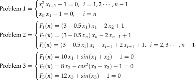
Problem 1=
(
x2
i xi+1−1=0, i=1, 2· · ·,n−1
xnx1−1=0, i=n
Problem 2=
F1(x) = (3−0.5x1)x1−2x2+1
F2(x) = (3−0.5xn)xn−2xn−1+1
Fi(x) = (3−0.5xi)xi−xi−1+2xi+1+1, i=2, 3· · ·,n−1
Problem 3=
F1(x) =10x1+sin(x1+x2)−1=0
F2(x) =8x2−cos2(x3−x2)−1=0
F3(x) =12x3+sin(x3)−1=0
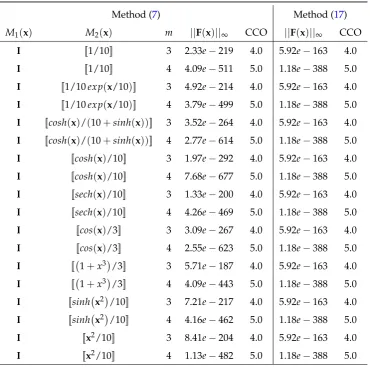
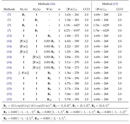
Tables1,2, and3clearly show that the claimed orders of convergence are in agreement with computational orders of convergence for a given number of steps. The simulation times in each Table for all the conducted tests are almost equal. In Table3, we have used full matrices as preconditioners because the system of nonlinear equations is small. But for a large system of nonlinear equations, it is not recommendable to use full matrices as a preconditioners and reason is clear, since we get a penalty in terms of computational cost. One of the main targets of the present article is to explore different possibilities of preconditioning, by keeping the convergence order. In our analysis, we found that for solving system of nonlinear equations, the iterative method (7) is the most efficient when we use the preconditioning matricesM1(x)andM2(x)as diagonal matrices. It is also observed that the
leading constant coefficients of preconditioners should be less one in magnitude to get better accuracy. The proposed iterative methods show better accuracy compared with multi-step Newton method for almost all tests, when considering the previous three model problems.
Table 1.Problem 1: Initial guess:xi=15/10,n=200, Iter= 5
Method (7) Method (17)
M1(x) M2(x) m ||F(x)||∞ CCO ||F(x)||∞ CCO
I [[−sin(x)/(1.1+cos(x))]] 1 2.97e−23 2.0 3.20e−7 1.99
I −I 2 1.95e−127 4.0 4.15e−28 3.0
I [[−2exp(−2x)]] 3 7.20e−89 4.0 5.56e−80 4.0 I [[−exp(−x)]] 4 3.21e−221 5.0 3.20e−185 5.0
4. Conclusions
The computational cost of the classical multi-step Newton method and that of the proposed iterative methods are substantially tre same, if we do not use dense preconditioners. Indeed, the iterative method (7) is more effective, when coupled with diagonal preconditioners. The proposed family of iterative methods has the same convergence order as that of Newton multi-step iterative method, with almost the same computational cost. The only assumption on the preconditioners is that they should have finite norms, in their definition domain.
Author contributions: First author established the idea and all other authors contributed equally in the article.
Table 2.Problem 2: Initial guess:xi=−1,n=100, Iter= 4
Method (7) Method (17)
M1(x) M2(x) m ||F(x)||∞ CCO ||F(x)||∞ CCO
I [[1/10]] 3 2.33e−219 4.0 5.92e−163 4.0
I [[1/10]] 4 4.09e−511 5.0 1.18e−388 5.0
I [[1/10exp(x/10)]] 3 4.92e−214 4.0 5.92e−163 4.0 I [[1/10exp(x/10)]] 4 3.79e−499 5.0 1.18e−388 5.0 I [[cosh(x)/(10+sinh(x))]] 3 3.52e−264 4.0 5.92e−163 4.0 I [[cosh(x)/(10+sinh(x))]] 4 2.77e−614 5.0 1.18e−388 5.0 I [[cosh(x)/10]] 3 1.97e−292 4.0 5.92e−163 4.0 I [[cosh(x)/10]] 4 7.68e−677 5.0 1.18e−388 5.0 I [[sech(x)/10]] 3 1.33e−200 4.0 5.92e−163 4.0 I [[sech(x)/10]] 4 4.26e−469 5.0 1.18e−388 5.0 I [[cos(x)/3]] 3 3.09e−267 4.0 5.92e−163 4.0 I [[cos(x)/3]] 4 2.55e−623 5.0 1.18e−388 5.0
I [[ 1+x3
/3]] 3 5.71e−187 4.0 5.92e−163 4.0
I [[ 1+x3
/3]] 4 4.09e−443 5.0 1.18e−388 5.0 I [[sinh x2
/10]] 3 7.21e−217 4.0 5.92e−163 4.0 I [[sinh x2
/10]] 4 4.16e−462 5.0 1.18e−388 5.0
I [[x2/10]] 3 8.41e−204 4.0 5.92e−163 4.0
Table 3.Problem 3: Initial guess:xi=15/10,n=3, Iter= 8
Methods (16) Method (17)
Methods M1(x) M2(x) V(x) m ||F(x)||∞ CCO ||F(x)||∞ CCO
(7) R1 I - 1 1.63e−241 2.0 6.69e−268 2.0
(7) I R1 - 1 1.34e−281 2.0 6.69e−268 2.0
(7) R1 I - 2 1.19e−6427 3.0 1.74e−6229 3.0
(7) I R1 - 2 4.27e−8197 3.0 1.74e−6229 3.0
(13) I I R2 1 1.49e−272 2.0 6.69e−268 2.0
(14) [[F(x)]] I 0.001R2 1 4.43e−290 2.0 6.69e−268 2.0
(14) [[F(x)]] I 0.001R3 1 2.22e−283 2.0 6.69e−268 2.0
(14) [[F(x)]] I 0.001R4 1 1.25e−286 2.0 6.69e−268 2.0
(14) I [[F(x)]] 0.001R2 1 2.84e−270 2.0 6.69e−268 2.0
(14) I [[F(x)]] 0.001R3 1 3.11e−270 2.0 6.69e−268 2.0
(14) I [[F(x)]] 0.001R4 1 5.34e−273 2.0 6.69e−268 2.0
(15) [[−F(x)]] I R5 1 1.36e−278 2.0 6.69e−268 2.0
(15) I I R6 1 3.74e−296 2.0 6.69e−268 2.0
(15) I I R7 1 4.75e−300 2.0 6.69e−268 2.0
(15) I I R8 1 3.73e−334 2.0 6.69e−268 2.0
(15) I I R9 1 7.06e−325 2.0 6.69e−268 2.0
(15) I I R10 1 5.79e−303 2.0 6.69e−268 2.0
R1= (0.1exp(0.1x)) (0.1exp(0.1x))T,R2= [1, 0, 0]T,R3= [0, 1, 0]T,R4= [0, 0, 1]T
R5=0.001[−1,−1,−1]T,R6=0.001[1,−1, 1]T,R7=0.001[−1,−1, 1]T,R8=0.001[−1,−1, 2]T
References
1. J. M. Ortega, W. C. Rheinbodt, Iterative solution of nonlinear equations in several variables, United Kingdom: Academic press limited 24-28 Oval road, London NW1 7DX, 1970.
2. J. F. Traub, Iterative Methods for the Solution of Equations, Prentice-Hall, Englewood Cliffs, 1964. 3. R. L. Burden, J.D. Faires, Numerical Analysis. PWS Publishing Company, Boston, USA, 2001.
4. J. M. McNamee, Numerical Methods for Roots of Polynomials. Part I, Elsevier, Amsterdam, Holland, 2007. 5. M. Z. Ullah, F. Soleymani, A. S. Al-Fhaid, Numerical solution of nonlinear systems by a general class of
iterative methods with application to nonlinear PDEs, Numerical Algorithms, vol. 67, pp. 223-242, 2014. 6. H. Montazeri, F. Soleymani, S. Shateyi, S.S. Motsa, On a New Method for Computing the Numerical Solution
of Systems of Nonlinear Equations, Journal of Applied Mathematics, vol. 2012, Article ID 751975, 15 pages, 2012, doi:10.1155/2012/751975.
7. A. Cordero, M. Kansal, V. Kanwar, A stable class of improved second-derivative free Chebyshev-Halley type methods with optimal eighth order convergence ,Numer. Algor. 72, 937. 2016.
8. V. Arroyo, A. Cordero, J. R. Torregrosa, Approximation of artificial satellites’ preliminary orbits: The efficiency challenge, Math. Comp. Model. 54(7-8), 1802-1807, 2011.
9. D. A. Budzko, A. Cordero, J. R. Torregrosa, New family of iterative methods based on the Ermakov-Kalitkin scheme for solving nonlinear systems of equations, Comput. Math. and Math. Phys. 55, 2015.
10. S. Qasim, Z. Ali, F. Ahmad, S. S-Capizzano, M. Z. Ullah, A. Mahmood, Solving systems of nonlinear equations when the nonlinearity is expensive, Comput. Math. Appl. 71(7), 1464-1478, 2016.
11. U. Qasim, Z. Ali, F. Ahmad, S. S-Capizzano, M. Z. Ullah, M. Asma, Constructing Frozen Jacobian Iterative Methods for Solving Systems of Nonlinear Equations, Associated with ODEs and PDEs Using the Homotopy Method, Algo. 9(1), 2016.
12. A. Cordero, J. L. Hueso, E. Martinez, J.R. Torregrosa, A modified Newton-Jarratt’s composition, Numerical Algorithms, vol. 55, pp. 87-99, 2010.
13. F. Ahmad, E. Tohidi, J. A. Carrasco, A parameterized multi-step Newton method for solving systems of nonlinear equations, Numerical Algorithms, pp. 1017-1398, 2015.
14. M. Z. Ullah, S. Serra-Capizzano, F. Ahmad, An efficient multi-step iterative method for computing the numerical solution of systems of nonlinear equations associated with ODEs, Applied Mathematics and Computation, vol. 250, pp. 249-259, 2015.
15. F. Ahmad, E. Tohidi, M. Z. Ullah, J. A. Carrasco, Higher order multi-step Jarratt-like method for solving systems of nonlinear equations: Application to PDEs and ODEs , Computers & Mathematics with Applications, vol. 70, no. 4, pp. 624-636, 2015, http://dx.doi.org/10.1016/j.camwa.2015.05.012.
16. X. Wu, Note on the improvement of Newton’s method for systems of nonlinear equations, Applied Mathematics and Computation, vol. 189, pp. 1476-479, 2007.
17. J. L. Hueso, E. Martínez, J. R. Torregrosa, Modified Newton’s method for systems of nonlinear equations with singular Jacobian, Journal of Computational and Applied Mathematics, vol. 224, pp. 77-83, 2009. 18. M. A. Noor and F. A. Shah, A Family of Iterative Schemes for Finding Zeros of Nonlinear Equations having
Unknown Multiplicity, Appl. Math. Inf. Sci., vol. 8, no. 5, pp. 2367-2373, 2014.
19. M.A. Noor, M. Waseem, K.I. Noor, E. Al-Said, Variational iteration technique for solving a system of nonlinear equations, Optim. Lett., vol. 7, pp. 991-1007, 2013,doi 10.1007/s11590-012-0479-3.