Fluid-structure interaction analysis of gravity-based
structure (GBS) offshore platform with partitioned
coupling method.
IW.Z. Lima,∗, R.Y. Xiaob
aAdvanced Sustainable Manufacturing Technologies (ASTUTE), College of Engineering,
Swansea University, Swansea SA2 8PP, United Kingdom
bSchool of The Built Environment and Architecture, London South Bank University,
Borough Road, London SE1 0AA, United Kingdom
Abstract
Fluid structure interaction (FSI) analysis is of great significance with the ad-vance of computing technology and numerical algorithms in the last decade. This multidisciplinary problem has been expanded to engineering applica-tions such as offshore structures, dam-reservoirs and other industrial appli-cations. The motivation of this research is to investigate the fundamental physics involved in the complex interaction of fluid and structural domains by numerical simulations and to tackle the multiple surface interactions of a one-way coupling FSI GBS engineering case. To solve such problem, the partitioned method has been adopted and the approach is to utilise the ad-vantage of the existing numerical algorithms in solving the complex fluid and structural interactions. The suitability has been validated for both strong and weak coupling methods which are the distinctive partitioned coupling approach. Therefore, with the computational platform of ANSYS FEA, the coupled field methods were adopted in this numerical analysis. Comparisons were made with the results obtained to justify the ability of both strong and weak methods in resolving the one-way coupling example with the potential applications in the field of ocean and marine engineering.
Keywords: fluid-structure interaction, offshore structure,partitioned
IFully documented templates are available in the elsarticle package on CTAN.
∗W.Z. Lim
method
1. Introduction
Fluid structure interaction is a complex multi-physics phenomenon with contiguous domains consisting generally on fluid flow and solid structures with interaction between them. The structure deforms due to fluid action; mainly pressure and viscous stress. FSI has become a crucial consideration 5
in the design of offshore structure engineering either from the research or in-dustry applications such as offshore structures (Jo et al., 2013), wind turbine (Zhang et al., 2014) and ship structure (Ma and Mahfuz, 2012). The com-plexity of the offshore structures under a challenging environment of high sea-water pressure impact has led to the development of robust numerical solvers 10
for fluid-structure interaction problems. The numerical methods can be dis-tinguished as either monolithic or partitioned method. In the monolithic approach, the interaction between the fluid and structure domain is treated synchronously under the interaction domain and are discretized in time and space in the same manner. Information is exchanged on the interface syn-15
chronously and this single solution equation can be solved simultaneously for the fluid flow and displacement of the structure implicitly. This fully-coupled or direct approach is known to be highly robust and stable for a very strong fluid-structure interaction analysis such as in the research (Michler et al., 2004) and (Walhorn et al., 2005). However, monolithic method represents 20
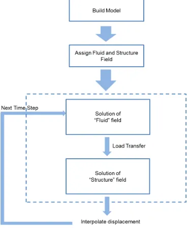
less modularity and require more coding than partitioned approach in which flow and structural equations are solved by using independent suitable algo-rithms and discretization methods. The partitioned method is an approach of which the two distinctive solvers (fluid and structure) are solved separately for the fluid flow and the displacement of a structure. The fluid and struc-25
ture equations are integrated in time and the interface conditions are enforced asynchronously which means that the fluid flow does not change while the so-lution of the structural equations is calculated and vice versa. This approach preserves the software modularity and requires a coupling algorithm to al-low for the interaction and to determine the solution of the coupled problem 30
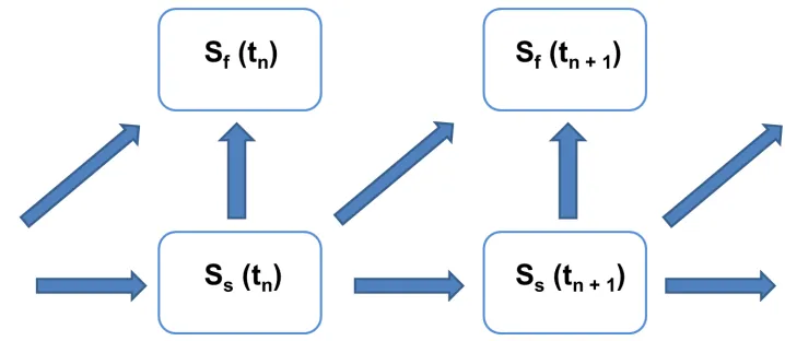
considered in the case of a single directional load which affects only from a particular field to another, for an example the fluid, Sf and the structure, Ss
interaction of one-way coupling system as shown in Fig. 1 below (Richter, 2010).
40
Fig. 1 Weakly coupled system for the one-way partitioned method
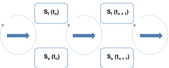
The interface between both domains is crucial and in most applications, a strong coupling system is approachable and this decoupling system allows parallel solution of the fluid and the structure domains. A strongly coupled system is a further development of the partitioned approach that two domains are solved independently in a decoupled way with an iterative interaction 45
loop between each time-steps as indicated in Fig. 2. One advantage of the partitioned approach is that different solvers and schemes can be used for different multi-physics fields such as Habchi et al. (2013)Degroote et al. (2010)Song et al. (2013)Wall et al. (2007)Dettmer and Peri (2008).
2. Mathematical model
50
The governing equations of fluid and structural mechanics are presented in association with the Finite Element Method, Lagrangian Formulation and the Arbitrary Lagrangian-Eulerian formulation. These computational tech-niques are further implemented in solving the environment of the offshore FSI analysis solution within the framework of ANSYS APDL.
Fig. 2 Strongly coupled system for the one-way partitioned method
2.1. Governing equations of fluid mechanics
The fluid flow is defined by the laws of conservation of mass, momentum, and energy. Such laws are expressed in terms of partial differential equations which are discretised through finite element scheme ANSYS (2013). The fluid flow equations are governed by Navier-Stokes equations of incompressible 60
flow.
2.1.1. Continuity equation
The continuity equation of the fluid flow is shown as:
∂ρ
∂t +∇·(ρv) = 0, (1)
where v is the velocity vectors for component in the x, y and z directions. ρ
is the density of the fluid and t is the time shown in the equation above. The rate of change of density can be replaced by the rate of change of pressure:
∂ρ ∂t =
∂ρ ∂P
∂P
∂t. (2)
As for the incompressible solution:
dρ dP =
1
β, (3)
2.1.2. Momentum equation 65
In a Newtonian fluid, the relationship between the stress and rate of deformation of the fluid is shown as:
τ = [λtr (∇u)−P]I+µ ∇u+∇uT
, (4)
whereτ,P,u,µandλrepresent the stress tensor, the fluid pressure, orthog-onal velocity vectors, dynamic viscosity and second coefficient of viscosity, respectively. The product of the second coefficient of viscosity and the di-vergence of the velocity is zero for a constant density fluid. Equation (4) transforms the momentum equations to the Navier-Stokes equations as fol-lows:
∂ρv
∂t +∇·(ρv⊗v) =ρg−P +R+∇·(µe∇v) +T, (5)
where g, R and T represent the acceleration vector due to gravity, dis-tributed resistances and viscous loss terms vectors. The density of the fluid properties and effective viscosity are presented asρ andµe respectively. The
viscous loss terms vector, T for all coordinate directions are eliminated in the incompressible, constant property case. The order of the differentiation 70
is reversed in each term, reducing the term to a derivative of the continuity equation, which is zero.
2.1.3. Turbulence
Turbulence occurs when the inertial effects are significant enough with respect to viscous effects and the instantaneous velocity being fluctuate at every point in the flow field. The velocity is thus expressed in terms of a mean value and a fluctuating component:
Vx = ¯Vx+V 0
x, (6)
where ¯Vx andV 0
x are the mean component of velocity and fluctuating
compo-nent of velocity in x-direction respectively. In the Navier-Stokes equations, the instantaneous velocity equation is time averaged where the fluctuating component is zero and the time average of the instantaneous value is the average value. The time interval for the integration is arbitrarily chosen as shown below:
1 ∆t
Z δt
0
Vx0dt= 0; 1
δt
Z δt
0
After the substitution of Equation (6) into the momentum equations, the time averaging leads to additional terms and the extra terms are:
σR=−∇ ·(ρV0⊗V0) (8)
where σR is the Reynolds stress terms. The standard k-model is applied
where the turbulent viscosity,µtis calculated as a function of the turbulence
parameters kinetic energy k and its dissipation rate using the Equation (9) below where Cµ is the turbulence constant and is the turbulent kinetic
energy dissipation rate.
µt=Cµρ
k2
. (9)
2.1.4. Pressure
For the calculation of the pressure, the defining expression for the relative pressure is:
Pabs =Pref +Prel−ρo·g·r+
1
2ρo(ω×ω×r)·r. (10)
Combining the momentum equations into vector form, the result is obtained as:
ρDν
Dt + 2ρω×ν +ρω×ω×r =ρg−∇Pabs+µ∇·(∇ν), (11)
where ρo, Pref, g, Pabs, Prel, r, w, v,µ, and ρare the reference density,
ref-75
erence pressure, gravity vector, absolute pressure, relative pressure, position vector of fluid particle relating to rotating coordinate system, angular velocity vector, velocity vector in global coordinate system, fluid viscosity and fluid density respectively. For the case of coupling in fluid flow, moving interfaces are included with the effect on the structural deformation which will deform 80
the fluid mesh. Such phenomenon changes with time and needs to satisfy the boundary conditions at the moving interfaces, Arbitrary Lagrangian-Eulerian (ALE) formulation Donea and Huerta (2003) is applied in solving such problems and the examples can be found in Bathe and Zhang (2009).
2.1.5. Arbitrary Lagrangia-Eulerian, ALE algorithms 85
large distortions in the fluid motion and are indispensable for the simula-tion of turbulent flows. On the contrary, it has the difficulty to follow free surface(s) and interface(s) between different materials or different media for example the fluid to fluid and fluid to solid interfaces. Therefore, we have ruled out such algorithms rather than only considering the ideal Arbitrary Lagrangian-Eulerian algorithms as the key solution of fluid domain and the fluid-structure interfaces instead Donea and Huerta (2003). Fluid flow prob-lems often involve moving interfaces which include moving internal walls (for example, a solid moving through a fluid), external walls or free surfaces. ALE formulations are used to solve the problems where the fluid domain of the seawater changes with time and movement of finite element to satisfy the boundary conditions at the moving interface(s). The Eulerian equations of motion need to be modified to reflect the moving frame of reference. The time derivative terms are essentially rewritten in terms of the moving frame of reference where φ and W are the degree of freedom and velocity of the moving frame of reference, respectively as shown below:
δφ
δt |fixed frame = δφ
δt |moving frame −W ·∇φ. (12)
2.1.6. Segregation solution algorithm
For coupling algorithm, the pressure and momentum equations are cou-pled with the SIMPLEF algorithm originally belong to a general class referred to as the Semi-Implicit Method for Pressure Linked Equations (SIMPLE), see Versteeg and Malalasekera (2007). The incompressible algorithm is a spe-90
cial case of the compressible algorithm. The change in the product of density and velocity from each iteration is approximated by the considering changes separately through a linearization process as shown in ANSYS (2013):
2.2. Governing equations of structural mechanics
The offshore structure equation is based on the impulse conservation that is solved by using a finite element approach as shown below whereM,C,K,
¨
u,u˙ anduare the mass, damping coefficient, stiffness, acceleration, velocity, and displacement vectors, respectively:
M ·u¨+C·u˙ +K ·u=F. (13)
2.2.1. von Mises yield criterion 95
variable for causing yield of materials which are pressure-independent. The von Mises or equivalent strain εe is computed as:
εe =
1 1 +ν0
1 2
(ε1−ε2) 2
+ (ε2−ε3) 2
+ (ε3−ε1) 2
12
, (14)
where ε1, ε2 and ε3 are the three principal strains and ν
0
is the effective Poisson’s ratio. The equivalent stress (von Mises) related to the principal stress can be obtained from
σe =
1 2
(σ1−σ2)2 + (σ2−σ3)2+ (σ3 −σ1)2
12
(15)
or
σe =
1 2
(σx−σy)
2
+ (σy−σz)
2
+ (σz−σx)
2
+ 6 σxy2 +σyz2 +σxz2
12
,
(16)
where σe is the equivalent stress of any arbitrary three-dimensional stress
state to be represented as a single positive stress values. The equivalent stress is part of the maximum equivalent stress failure theory known as yield functions which can be referred to Chen (2007). When ν0 =ν the equivalent stress is related to the equivalent strain through
σe=Eεe. (17)
2.3. Coupling equations
The interaction of the fluid seawater and the offshore structure at a mesh interface causes the pressure to exert a force applied to the structure and the structure motions produce an effective fluid load. The governing finite element matrix equations then become:
[Ms]U¨ + [Ks]U¨ =Fs+ [R]P
[Mf]P¨+ [Kf]P¨ =Ff −ρo[R] T ¨
U, (18)
The coupling matrix [R]also takes into account the direction of the normal vector defined for each pair of coincident fluid and structural element faces that comprises the interface surface. The positive direction of the normal vector, as the program uses it, is defined to be outward from the fluid mesh and inwards to the structure. Both the structural and fluid load quantities that are produced at the fluid-structure interface are functions of unknown nodal degrees of freedom. Placing these unknown load quantities on the left hand side of the equations and combining the two equations into a single equation produces the following:
Ms 0
ρoRT Mf
¨ U ¨ P +
Ks −R
0 Kf U P = Fs Ff . (19)
The foregoing equation implies that nodes on a fluid-structure interface have both displacement and pressure degrees of freedom.
100
3. Gravity based offshore structure, GBS platform
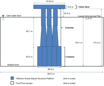
The offshore gravity-based structure (GBS) platform was modelled which was based on the MARINTEK, Norway three dimensional model Stansberg et al. (2005) Baarholm and Stansberg (2004). The aim of this three dimen-sional numerical analysis was to understand the behaviour of the offshore 105
structure and to further validate the suitability of both strong and weak par-titioned coupling methods and to make comparison that involved multiple interaction surfaces. The GBS platform was coupled with the attempt of both strong and weak coupling techniques undergo high wave impact from the recent Tohoku, Japan, 2011 earthquake that induced a high velocity in-110
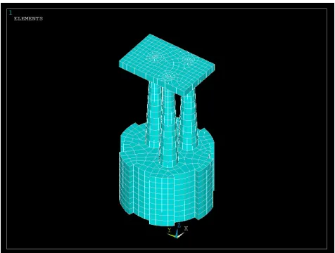
flow. The actual recorded peak acceleration of 26.49m/s2att=1.10 s Kalkan and Sevilgen (2011) was taken having the peak velocity of 29.99m/s. The hypothetical model of the GBS platform can best be referred to Fig. 3 and the material properties of the offshore structure GBS platform was assumed as a high strength concrete with the properties stated in Table 1 as shown. 115
Fig. 3 Hypothetical model of the offshore gravity-based structure (GBS) platform (the Statfjord A GBS platform, North Sea) from MARINTEK, Norway and the sea-water level.
and weak coupling system will be compared in respective to hydrodynamics pressure and von Mises stress obtained in the later section.
4. Numerical model
In the computational application of the GBS offshore structure, ANSYS APDL was chosen to be the computing platform where the corresponding 125
element types that were used are element SOLID185 for the offshore GBS platform and element FLUID142 for the sea water under high wave impact fluid flow domain. The SOLID185 element is defined as eight nodes hav-ing three degrees of freedom at each node: translations in the nodal x, y, and z directions. Whereas the FLUID142 element is defined by eight nodes 130
Table. 1 Materials properties for the gravity-based offshore structure, GBS
Material Elastic Modulus Poisson Ratio’s Density Viscosity (MPa) (kg/m3) (P a.s)
Concrete (High-Strength) 30 0.2 2400
-Water - - 1000 8.9
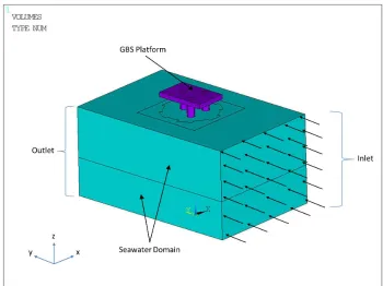
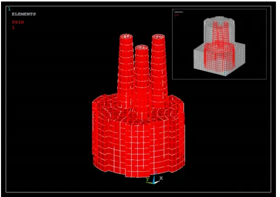
FLUID142 elements are compatible in relation to the coupled-field method of fluid interacting with the solid structure in three dimensional forms.
Fig. 5 Three-dimensional numerical model of the sea-water domain (FLUID142 elements).
The geometry of the numerical model of the GBS platform and seawater is depicted in Fig. 4. The inlet velocity vector was assigned at the y-direction 135
in the global coordinate system. Three dimensional SOLID185 elements provide the degree of freedom of deformation and von Mises stress in the discipline of structure analysis solver and FLUID142 elements provide the degree of freedom of velocity and hydrodynamics pressure in the discipline of FLOTRAN-CFD analysis solver. The element model and offshore GBS 140
platform domain are illustrated in Fig. 5 and Fig. 6 respectively.
4.1. Coupling methods
The partitioned approach of coupling methods Multi-Field Single-Code, MFS and Load Transfer Physics Environment adapted in the ANSYS APDL platform are considered and compared for this numerical FSI problem. Such 145
coupling methods had also been adopted by Lim et al. (2012) and Lim et al. (2013) for the problem of concrete gravity dam. The MFS coupling solver is specified as strong coupled system of partitioned method and the solution method is specifically shown in Fig. 7. It can be defined as a sequential coupled field system that is able to solve a lot of coupling analysis prob-150
lems. The MFS solver was defined with twenty time-steps and within each time loop there is a stagger loop. The staggering loop allow for implicit coupling of the seawater and offshore structure fields in the MFS solution. The maximum twenty iterations of stagger iteration specified are to deter-mine the convergence of the load transfer between fields. The displacement 155
Fig. 7 Solution procedure of Multi-Field Single-Code coupling (MFS) for the FSI GBS offshore problem (Strong Coupling System).
The Load Transfer Physics Environment is consider as weak coupled sys-tem of partitioned method under a developed user looping syssys-tem with the 160
ANSYS parameter design language (APDL). The looping of the weak cou-pling system is shown in Fig. 8 and the input of one physics analysis de-pends on the results from another analysis. For the weak coupling system of Load Transfer Physics Environment, there is no staggering iteration between each time loop hence the solutions are easily converged within the maximum 165
twenty time-steps specified. In this paper, the numerical problem is treated as a one-way coupling approach and both methods involve the multiple sur-face interactions between the fluid and structural domain especially at the columns and base surfaces shown in Fig. 9.
5. Results and discussion
170
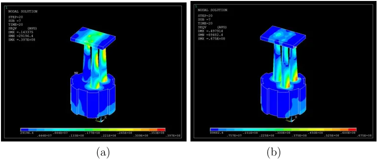
Based on the results of both coupled-field analyses, the distribution pat-terns of the hydrodynamics pressure and von Mises stress are fairly rational and agreeable for the offshore GBS numerical problem in terms of compar-ison. Such results was proven and shown in Fig. 10 for the hydrodynamics pressure of the sea water domain around the surface of the GBS offshore 175
platform base as well as the build-up von Mises stresses on the overall GBS Offshore structure as shown in Fig. 11 for the strong and weak coupling approach.
Five different node locations were selected on the morphing region (sea-water domain) and the offshore GBS structure domain as shown in Fig. 12 180
with the purpose of further verification and comparison of the both meth-ods. Comparison results of the average hydrodynamics pressure and von Mises stress values for the different node locations are shown in Fig. 13 and Fig. 14. It clearly show that the distribution patterns for the pressures and stresses of both methods were rationally similar and close in comparison for 185
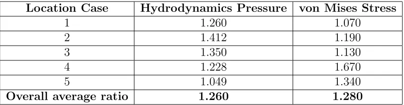
all the node locations. Such indicate that the both coupling system are ca-pable of solving high density of surface(s) interaction. In terms of value, the maximum average ratio for hydrodynamics pressure is 1.412 (Location Case 2) and for the von Mises stress is 1.670 (Location Case 4). The comparison results can best refer to Table 2 for better study on the overall average ra-190
Table. 2 Average ratio of hydrodynamics pressure and von Mises stress in com-parison of both MFS and Load Transfer Physics Environment methods for the offshore GBS platform
Location Case Hydrodynamics Pressure von Mises Stress
1 1.260 1.070
2 1.412 1.190
3 1.350 1.130
4 1.228 1.670
5 1.049 1.340
Overall average ratio 1.260 1.280
There were only a slight variations in the overall average ratio value be-tween the comparison of both coupling methods. Hence, regardless of the 195
(a) (b)
Fig. 10 Comparison of hydrodynamics pressure distribution results between (a) Multi-Field Single Code, MFS (Strong Coupling) and ; (b) Load Transfer Physics Environment (Weak Coupling) around the interaction surfaces at the GBS offshore platform base.
(a) (b)
(a) (b)
Fig. 12 Selected node locations of the (a) seawater (morphing region) domain on the hydrodynamics pressure results; (b) Offshore GBS platform on the von Mises stress results.
high stresses are of the same occurring at the bottom and sides of the 200
rigid concrete gravity-dam structure. Such results and analysis conclude that the overall one-way coupling could be resolved with the approach of both partitioned weak and strong coupling systems in the MFS and Load Transfer Physics Environment respectively. These proved that the weak and strong coupling methods are capable in solving the many problem of a one-205
way coupling offshore structure issue in carrying out feasibility design analysis especially under harsh pressure conditions .
6. Conclusions
The analysis of GBS platform used in this paper was to illustrate the differences between the coupling algorithms for both strongly and weakly 210
coupled user developed system of the partitioned methods. These will enable feasible applications in the area of offshore and marine engineering structures. The scope and capability of both methods have been tested and compared from the numerical results obtained, it has proved that both weak and strong coupled field methods are oscillating with the same pressure and stress distri-215
butions that justify their capabilities of transferring load between the surfaces of interaction. In both examples, the offshore structures have responded to the pressure impact through the interaction surface or region with the distri-bution patterns being similar. However, the small differences of average ratio in the stress value could be caused by the stringent convergence in the strong 220
coupling algorithm due to the multiple surface interactions of the numerical model whereas the weak coupling algorithm has loose convergence within the surface of interaction. The developed techniques of the weak coupling system has been proved to be more flexible in terms of the existing APDL in ANSYS which allow the development of parameters and algorithms proposed in this 225
paper in tackling the one-way coupling FSI GBS Offshore platform problem. Hence, the user assigned one-way weak coupling algorithm can be an ideal method in solving both single and multiple scale of surface interactions in a feasible design analysis of an offshore or marine engineering field.
Acknowledgements
230
References
235
ANSYS (2013). Documentation Release 14.5.
Baarholm, R. and Stansberg, C. T. (2004). Extreme vertical wave impact on the deck of a gravity-based structure (GBS) platform. Rogue Waves.
Bathe, K. J. and Zhang, H. (2009). A mesh adaptivity procedure for CFD and fluid-structure interactions. Computers & Structures, 87(1112):604 – 240
617.
Benra, F. K., Dohmen, H. J., Pei, J., Schuster, S., and Wan, B. (2011). A comparison of one-way and two-way coupling methods for numerical analysis of fluid-structure interactions. Journal of Applied Mathematics.
Chen, W. F. (2007). Plasticity in reinforced concrete. J. Ross Publishing. 245
Degroote, J., Haelterman, R., Annerel, S., Bruggeman, P., and Vierendeels, J. (2010). Performance of partitioned procedures in fluidstructure interac-tion. Computers & Structures, 88(78):446 – 457.
Dettmer, W. and Peri, D. (2008). On the coupling between fluid flow and mesh motion in the modelling of fluidstructure interaction. Computational 250
Mechanics, 43(1):81–90.
Donea, J. and Huerta, A. (2003). Finite element methods for flow problems. Wiley, England.
Habchi, C., Russeil, S., Bougeard, D., Harion, J. L., Lemenand, T., Ghanem, A., Valle, D. D., and Peerhossaini, H. (2013). Partitioned solver for 255
strongly coupled fluidstructure interaction. Computers & Fluids, 71(0):306 – 319.
Jo, C. H., Kim, D. Y., Rho, Y. H., Lee, K. H., and Johnstone, C. (2013). Fsi analysis of deformation along offshore pile structure for tidal current power. Renewable Energy, 54(0):248 – 252.
260
Lim, W. Z., Xiao, R., and Chin, C. S. (2012). A comparison of fluid-structure interaction methods for a simple numerical analysis of concrete gravity-dam. Proceedings of the 20th UK Conference of the Association for Com-265
putational Mechanics in Engineering .
Lim, W. Z., Xiao, R., T., H., and Chin, C. S. (2013). Partitioned meth-ods in computational modelling on fluid-structure interactions of concrete gravity-dam. Computer and Information Science.
Ma, S. and Mahfuz, H. (2012). Finite element simulation of composite ship 270
structures with fluid structure interaction. Ocean Engineering, 52(0):52 – 59.
Michler, C., Hulshoff, S., van Brummelen, E., and de Borst, R. (2004). A monolithic approach to fluidstructure interaction. Computers & Fluids, 33(56):839 – 848.
275
Richter, T. (2010). Numerical methods for fluid-structure interaction prob-lems. University of Heidelberg.
Song, M., Lefranois, E., and Rachik, M. (2013). A partitioned coupling scheme extended to structures interacting with high-density fluid flows. Computers & Fluids, 84(0):190 – 202.
280
Stansberg, C., Baarholm, R., Kristiansen, T., Hansen, E., and Rortveit, G. (2005). Extreme wave amplication and impact loads on offshore structures. Offshore Technology Conference.
Versteeg, H. and Malalasekera, W. (2007). An introduction to computational fluid dynamics the finite volume method. Pearson Education Limited, 285
England.
Walhorn, E., Klke, A., Hbner, B., and Dinkler, D. (2005). Fluid structure coupling within a monolithic model involving free surface flows. Computers & Structures, 83(2526):2100 – 2111.
Wall, W. A., Genkinger, S., and Ramm, E. (2007). A strong coupling parti-290