Machine Learning Based Network Analysis using
Millimeter-Wave Narrow-Band Energy Traces
Maria Scalabrin
†, Guillermo Bielsa
‡, Adrian Loch
‡, Michele Rossi
†, Joerg Widmer
‡Abstract—Next-generation wireless networks promise to pro-vide extremely high data rates, especially exploiting the so-called millimeter-wave frequency range. Gaining information from spec-trum usage is becoming important to provide smart adaptation capabilities to future network protocol stacks. Issues such as deafness, misaligned antennas, or blockage may severely impact network performance, and their identification is crucial. Despite the complexity of full analytical models, machine learning tech-niques are progressively being considered to improve spectrum usage at higher layers. In this paper, we design a signal processing technique that uses narrowband physical layer energy traces, obtained from one or multiple channel sniffers. The proposed technique utilizes a combination of template matching and an Explicit Duration Hidden Markov Model (EDHMM) to correctly classify frames, while coping with the non-stationarity of the traces. This leads to a protocol level monitor that does not need to decode the channel at the physical layer, but just infers the type of packets that are exchanged based on sub-sampled energy traces. The performance of this framework is evaluated using off-the-shelf mm-wave wireless devices, quantifying its detection performance in the presence of one or multiple sniffers, and assessing the impact of physical layer parameters such as noise power and signal levels.
Index Terms—millimeter-wave, Hidden Markov Model, phys-ical layer, energy traces, machine learning, protocol analyzer
I. INTRODUCTION
Next-generation wireless networks are called to provide extremely high data rates, especially exploiting the so-called millimeter-wave frequency range [1]. Applications and ser-vices will benefit from these high rates and the radio spectrum will become more and more densely utilized. As wireless networks turn into increasingly complex systems, accurate and scalable analytical models to characterize their behavior are not yet available and very challenging to obtain. Instead, a promising approach is provided by machine learning tools that learn from data [2]–[4]. Gaining information from spectrum usage is deemed important to provide smart adaptation capa-bilities to future network protocol stacks. Possible applications include: (i) channel diagnosis: detect communication problems such as a link blockage, (ii) Quality of Service (QoS) tracking and adaptation, i.e., efficiently manage channel resources ac-cording to the detected energy level, (iii) information security: discovery of malicious signaling messages, etc.
As for the millimeter-wave (mm-wave) channel, its direc-tional nature results in communication issues that strongly impact higher layers, but which are hard to identify without
†Department of Information Enginering, University of Padova,
via Gradenigo 6B, 35131 Padova, Italy. Email: {scalabri, rossi}@dei.unipd.it. ‡IMDEA Networks Institute, Avenida del Mar Mediterraneo 22, 28918 Leganes, Madrid, Spain. Email: {guillermo.bielsa,adrian.loch,joerg.widmer}@imdea.org.
detailed information of the underlying physical layer effects. This includes, e.g., deafness [5], misaligned antennas, and link blockage. Commercial Off-The-Shelf (COTS) devices are typically a black box regarding this physical layer information. As a result, troubleshooting COTS-based, real-world mm-wave network deployments often translates into time-consuming “trial-and-error” analysis. While understanding performance issues in such deployments is challenging [6]–[8], the resulting knowledge is extremely valuable. It provides useful insights for network planners and administrators. For instance, a miss-ing acknowledgment after a data packet hints at a deafness issue, overlapping packet frames suggest a collision, and so on. However, gaining such insights from a COTS node that forms part of the network is virtually impossible. On top of the aforementioned lack of lower-layer access, a single node would be restricted to its particular point of view—the directivity of the communication limits the insights that one could gain. To prevent this, we need to capture and compare the behavior of the network from multiple viewpoints. Given the extreme bandwidth available in mm-wave communications (e.g., 2 GHz per channel in the 60 GHz band), this requires an inordinate amount of data processing, and thus would be highly challenging.
In this paper, we start filling the above identified gaps through the design and evaluation of an automatic tool for mm-wave channel analysis based on COTS hardware. Specif-ically, the tool uses machine learning techniques to infer protocol-level details such as packet types, their energy level and duration, and can help detect performance bottlenecks in 60 GHz networks using narrowband physical layer energy traces from one or multiple (omnidirectional) sniffers. That is, we do not record and decode the full communication but only require the energy level that the sniffers receive.
bandwidth. Since we do not need to decode any of the data, our approach preserves privacy, works regardless of whether the network uses encryption, and does not require accurate time/frequency synchronization. As a result, the proposed technique is simple yet highly effective. Our contributions are summarized as follows:
• We design a machine learning framework based on tem-plate matching and an EDHMM to automatically infer protocol layer information, e.g., transmitted packet types, their energy and duration, in 60 GHz networks. The main challenge lies in the variability of the traces and in the complexity of identifying the structural elements in the traces given their noisiness, aperiodicity, and un-predictable behavior. Here, this is solved through a com-bination of statistical and machine learning techniques. • We introduce a time-adaptive learning mechanism to cope
with the non-stationarity of energy traces due to gain control adjustments and node movement. This run-time adaptation is barely explored in specialized work in the field of statistics but is critical for our approach. It also sets our scheme apart from existing work based on simple clustering or thresholding, which is highly sensitive to non-stationary behavior and thus often fails.
• We extend the learning framework to jointly process mm-wave channel traces from multiple time-synchronized sniffers. The idea is that different viewpoints of the same channel can provide diverse information and lead to higher decoding accuracies. • We evaluate our approach in an extensive measurement
campaign using COTS 60 GHz hardware to analyze its performance in a range of practical scenarios. Besides, we numerically quantify the ability of the framework to correctly identify protocol sequences (beacon pairs, data and acknowledgment frames) from single and multiple channel sniffers, looking at the impact of channel noise and its distribution across different sniffers.
This paper is organized as follows. The related work is surveyed in Section II. In Section III, we discuss typical IEEE 802.11ad energy traces. Some mathematical background on the standard HMM and the extended EDHMM framework is provided in Section IV. The machine learning framework is introduced in Sections V, VI, VII and VIII. In Section IX, this framework is generalized to perform decoding from multiple sniffers and a mm-wave channel trace generator that helps to evaluate the accuracy of our approach is presented in Section X. We finally evaluate the proposed technique using experimental and simulated energy traces in Section XI and provide some concluding remarks in Section XII.
II. RELATED WORK
In the following, we give an overview of performance analy-sis and troubleshooting in mm-wave networking. As sketched in Section I, mm-wave networks suffer from high path-loss and high absorption. To overcome this, nodes typically use directional antennas and Line-Of-Sight (LOS) paths. However, this makes links very susceptible to blockage. State-of-the-art work in this field [10]–[12] focuses on correctly identifying such blockage at the nodes involved in the communication,
and reacting in a timely manner. For instance, BeamSpy [11] measures the set of available paths between a transmitter and a receiver. This “path skeleton” serves as a reference whenever blockage occurs—the nodes compute which of the paths in the skeleton is most likely to be unaffected by the blockage and steer their antennas accordingly. As a result, BeamSpy can avoid costly beam steering overhead. Further, earlier work by the same authors [12] looks into differentiating device movement from blockage based on Received Signal Strength (RSS) measurements. This is key to ensure that nodes react correctly when links degrade. Similarly, MOCA [10] transmits a very short control message to assess the link state. If the transmitter does not obtain a reply, it assumes that the anten-nas are misaligned. Otherwise, it adapts the Modulation and Coding Scheme (MCS) according to the current channel state. All of the above approaches aim at improving the performance of mm-wave networks. In contrast, our worktroubleshootsthe operation of such approaches and is thus orthogonal to them. While BeamSpy and MOCA also try to identify specific issues in the communication, they are constrained to the specific “viewpoint” of a certain node. Our framework runs on one or more external sniffers which we can place at multiple locations, thus providing richer insights. Earlier work proposes an equivalent concept based on external sniffers. However, such approaches typically consider lower frequency bands, and focus on security issues [13], [14] such as realizing an Intrusion Detection System (IDS). The key difference to our study is that such security sniffers are designed to continuously operate along with the network, thus increasing the complexity of the deployment. In contrast, our tool does not need to be part of the network, and can be used on-demand only. Hence, we do not add complexity to the network. Moreover, we focus on performance issues in directional wireless networks while the above work deals with security in the omni-directional case. However, [14] and references therein also deal with raw physical layer data, similarly to our case. Specifically, they suggest overhearing the communication and jamming unwanted packets based on, for instance, header information. Our narrow band sniffer for wide band signals also overhears the communication but does not (and in fact cannot) decode any preambles and headers to identify the packets. Instead, we use machine learning on the timing of frames from simple energy traces to obtain the information required for network analysis.
ma-chine learning based solutions for spectrum sensing/sharing in Cognitive Radio (CR) represent a promising approach for improving the utilization of the radio electromagnetic spectrum [17], [18]. To promote this, the Defence Advance Research Projects Agency (DARPA) [19] intends to develop technologies for extensive spectrum sensing/sharing, both in the Radio Frequency Machine Learning Systems (RFMLS) program [2] as well as in another major DARPA effort known as the Spectrum Collaboration Challenge (SC2) [3], which is regarded as the first-of-its-kind collaborative machine-learning competition to overcome spectrum scarcity. Also the Na-tional Science Foundation (NSF) [4] is promoting projects to leverage machine learning solutions in CR. In the literature, automatic network recognition offers a promising framework for the integration of cognitive concepts at the network layer, bearing similarities with the mm-wave channel analyzer pro-posed in Section V. In [20], the authors address the problem of automatic classification of technologies, with particular focus on Wi-Fi vs. Bluetooth recognition. Previous work, as for example [21], has addressed a related problem, allowing cooperative spectrum sensing in peer-to-peer cognitive net-works by using distributed detection theory [22] for identifying overlapping air interfaces based on time-frequency analysis and feature extraction. The same problem is tackled in [23], where two kinds of neural classifiers are adopted. Again, the authors focus on Wi-Fi vs. Bluetooth recognition. While this work is related to ours, none of these studies perform protocol analysis from narrow band channel traces. We remark that our tool is the first automatic classifier of IEEE 802.11ad energy traces for network diagnosis. The uniqueness of our approach prevents direct comparison with earlier work.
III. ALOOK INTOIEEE 802.11AD ENERGY TRACES The IEEE 802.11ad standard operates at 60 GHz. In this band, propagation conditions are worse than at lower bands, such as at 2.4 or 5 Ghz, which are used by the IEEE 802.11n/ac standards [24]. Specifically, the path loss is much higher at60GHz than at2.4or5GHz. To compensate for this attenuation, IEEE 802.11ad provides a mechanism for the establishment of a directional communication link between a transmitter/receiver pair using a beam training process. As a result of this process, the transmitting station focuses its energy towards the intended receiver. This compensates for the high path loss and reduces the potential interference to other stations that are located nearby.
IEEE 802.11ad divides the channel access into so called Beacon Intervals (BIs). Each BI is split into different access periods, which have different access rules and provide specific functionalities to the stations (STAs) within communication range. A typical BI is composed of a Beacon Header In-terval (BHI) and a Data Transmission InIn-terval (DTI). The BHI contains several sub-intervals and is basically used to transmit control messages, such asbeacons that enable beam training. In the DTI period, STAs exchange data frames either exploiting a contention-based access period or a scheduled service period. The former entails a contention mechanism (“floor acquisition”) to acquire the medium, which uses the enhanced distributed coordination function. Conversely, in the
250 500 750 1000 1250 1500
Sample number 0
0.1 0.2 0.3
Amplitude [V]
Control Packets
(Beacon Pair) Data Packet and Acknowledgment Exchanges
Fig. 1. Energy trace example: DATA/ACK burst.
scheduled service period, stations access the channel in a contention-free manner.
An example IEEE 802.11ad energy trace corresponding to a data exchange is shown in Fig. 1. This trace depicts the start of a typical data burst. The data burst starts with a pair of beacons which contain control information. This pair of beacons is followed by a sequence of data (DATA) packets and acknowledgments (ACKs). In general, each DATA packet is followed by a corresponding ACK, which is the shorter packet in the figure and which has a higher energy level. Note that the higher amplitude of ACKs is due to the position of the sniffer, which in this case was near the receiver. The beam training process is composed of the following two phases.
• Sector Level Sweep (SLS). During the SLS, a STA selects acoarse grain antenna sector. This phase can be implemented in two ways: 1) through a transmit sector sweep (TXSS), i.e., a STA tries to select the best transmit antenna sector towards a particular receiving STA by transmitting Sector Sweep (SSW) frames using each of its antenna sectors or 2) through a receive sector sweep (RXSS), i.e., a receiving STA trains its receive antenna sector by requesting its peer STA to transmit SSW frames using a fixed antenna pattern, while the receiving STA sweeps across its receive antenna sectors.
• Beam Refinement (BR). To refine the sectors obtained in the SLS phase, multiple mechanisms are used. Basically, the two communicating STAs iteratively search for the optimal alignment starting from the coarse grain sector provided by the SLS. Occasional BR sequences retrain the antenna beams in case of, e.g., mobility, to ensure that both nodes remain in the boresight of each other. Sequences of control packets are not difficult to identify within IEEE 802.11ad channel traces. The SLS sweeps that are used during the connection setup have32different energy levels. The BR sequences, which are used for re-alignement, e.g., when there is a drop in the link quality, have 35 levels [25]. The particular number of energy levels depends on the number of sectors of the antenna. Existing hardware implements the above number of sectors. An example energy trace corresponding to a BR phase is shown in Fig. 2.
2 2.2 2.4 2.6 Time [s] ×10-3
0 0.02 0.04 0.06 0.08 0.1
Amplitude [V]
SN1
2 2.2 2.4 2.6 Time [s] ×10-3 -1
-0.5 0 0.5 1
Correlation
Fig. 2. Example IEEE 802.11ad beam refinement sequence (35energy levels, top) and correlation coefficient (bottom) with respect to the beacon template.
2 2.2 2.4 2.6 Time [s] ×10-3 0
0.02 0.04 0.06 0.08 0.1
Amplitude [V]
SN1
2 2.2 2.4 2.6 Time [s] ×10-3 -1
-0.5 0 0.5 1
Correlation
Fig. 3. Beam Refinement (BR) sequence of Fig. 2 (top) and corresponding correlation coefficient (bottom) with respect to the beacon template. A correlation threshold (horizontal line in the bottom plot) is used to single out beacon messages (top graph), whereas the inter-beacon distance reveals whether a beacon is part of the BR sweep. The BR sequence has35energy levels and is correctly identified, see the green line in the top plot.
when communicating at multi-gigabit-per-second rates. At the same time, recognizing frame types in an automated manner is hard. In this paper, our goal is to devise and validate a technique for the automatic identification and labeling of IEEE 802.11ad energy traces. Notably, BR/SLS sweeps can be reliably identified through a standard pattern matching tech-nique, as we briefly describe next. Each sequence is composed of beacon frames, each having a different energy level, but all of them having the same (although noisy) distinctive shape. To capture this shape, we obtained a beacon template, that is basically a smoothed out version of the beacons that were measured experimentally. Hence, a standard convolution is performed between the input energy trace and the beacon template; for an example see the bottom plot in Fig. 2. As we show in Fig. 3, setting a proper threshold on the correlation signal allows one to single out the start of each beacon in the original sequence. It is then not difficult to check when exactly 32 or 35 properly spaced energy levels appear in a
row and, in turn, detect the SLS/BR sweeps, see again Fig. 3. Further details on the template matching procedure are given in Section VI, whilst additional results on BR sequence detection are provided in Section XI-A.
While the identification of SLS/BR sweeps is doable through simple processing techniques, the characterization of DATA exchange phases is much more complex. In this case, we do not know in advance the duration of DATA frames. Similarly, we do not know the number of DATA/ACK exchanges in the data burst. There may be missing ACKs and the energy levels of ACKs and DATA frames can be arbitrary, as they depend on the location of the sniffer with respect to the transmitter and the receiver. In addition, the start of each data burst has to be reliably identified, and the start and end points of each frame transmitted therein have to be reliably assessed as well. All of this leads to a sequential estimation problem that is the subject of the work that we expound in the following sections.
IV. EDHMMPRELIMINARIES
Next, some mathematical background on the standard HMM and the extended EDHMM framework is provided as a basis for the machine learning framework, which is introduced in Sections V, VI, VII and VIII. Specifically, we demonstrate how the standard HMM is inadequate for our purpose. Still, we use it to calibrate the initial EDHMM.
We use uppercase and calligraphic fonts for sets, except for
N(X;µ, σ2), which refers to a Gaussian random variableX
with meanµand varianceσ2. We denote a random sequence of lengthTbyX1:T = (X1, . . . , XT), where the random variable Xtat time indext∈ {1, . . . , T}takes values in the setX, with
cardinality|X |. Realizations are indicated by lowercase letters, i.e.,xtis the realization ofXt, and withx1:T = (x1, . . . , xT) we denote a sequence of realizations. Vectors are indicated by bold letters, e.g.,bbb, and we refer to their elements asbbb= [b1, . . . , bK], with |bbb| = K. For matrices we use uppercase bold letters, e.g.,AAA={aij} is a matrix with elementsaij.
Markov models, whose states correspond to observable events, are inadequate to solve our mm-wave channel estima-tion problem. The reason is that we measure a noisy version of the transmitted energy levels, as they are corrupted by random channel fluctuations. Instead, Hidden Markov Models (HMMs) [26] are a more appropriate tool, as their observations are probabilistic functions of the (hidden) state. Specifically, an HMM is composed of embedded stochastic processes, where an unobservable hidden random process is revealed to the observer through another set of random processes that produce the sequence of observations.
We now consider a data burst and aim to solve the fol-lowing estimation problem. The observed channel samples in the data burst, O1:T = (O1, . . . , OT), are modeled as a
sequence of real-valued random variables corresponding to one of the following basic elements: “1” inter-frame space (IFS), “2” data packet (DATA) and “3” acknowledgement (ACK). Accordingly, the hidden stateStat timetis a discrete
t ∈ {1, . . . , T}. Our objective is then to reliably estimate the sequence of hidden states s1:T = (s1, . . . , sT) from observations o1:T = (o1, . . . , oT). The standard HMM makes two basic assumptions regarding the embedded stochastic processes:
A1) The first assumption is thatS1:T is a first-order Markov chain, i.e., P(St+1|S1, . . . , St) = P(St+1|St). In par-ticular, we have P(St+1 = j|St = i) = aij, where A
A
A = {aij}, i, j ∈ S, is the single-step transition
probability matrix of the HMM.1
A2) The second assumption is that the random variableOtis statistically independent of (O1, . . . , Ot−1).2
Moreover, Ot is a probabilistic function of the hidden state
St, i.e., it obeys a suitable conditional probability P(Ot|St) and each random variable Ot can use a private distribution
P(Ot|St)over the hidden state. We use a Gaussian observation
model with P(Ot|St=i) =N(Ot;µi, σi2), whereµi andσ2i
specify the mean and the variance of the random variable Ot, given that the hidden state is i ∈ S. This is known to well approximate the noise distribution for mm-wave channels [27]. For all hidden states i ∈ S, we collect the parameter pairs
bi = (µi, σ2
i) through vector bbb = [b1, . . . , b|S|]. We define
π π
π= [π1, . . . , π|S|], whereπi is the probability that the HMM is in state i∈ S in the first time slot of the burst.
The HMM model is described through a further parameter vectorΘ= [πππ, AAA, bbb]. Its maximum likelihood estimate given a sequence of observations is obtained through the Expectation-Maximization (EM) algorithm [28], which entails two-step iterations. Briefly, initial values for Θ are chosen, and using assumptions A1 and A2 the posterior distribution for the whole sequenceP(S1:T|O1:T,Θ)is computed. Hence, this posterior
is used to compute the expected log-likelihood (the Baum’s auxiliary function), Q(Θnew,Θ), as
Q(Θnew,Θ) =X
S1:T∈ST
P(S1:T|O1:T,Θ) logP(S1:T, O1:T|Θnew),
(1) which is finally maximized with respect to Θnew, where
Θnew is the new parameter vector (HMM model) from the EM iteration. This process is repeated until convergence to a local maximum. A proper initialization of Θ (with particular regard for bbb) is crucial for a good convergence of the EM algorithm. For a Gaussian-observation model, applying the two-step iterations of the EM algorithm is equivalent to using Baum’s re-estimation approach [29], which is as follows. Consider two new variables ξt(i, j) andγt(i), withi, j ∈ S, that are defined as ξt(i, j) =P(St=i, St+1=j|O1:T,Θ)
1Conversely, in the extended EDHMM, the entire process is not Markovian
(memoryless). Instead the process is Markovian only at specified time instants.
2Specifically, one observation per state is assumed in the standard HMM
model while in the EDHMM each state emits a sequence of observations. The length of the sequence while in statei∈ Sis determined by the length of time spent in statei∈ S, i.e., the durationd. Observations are assumed to be independent of timet, while in statei∈ S. Also, in the extended EDHMM, the transition probabilityaijis independent of the durationdof statei∈ S and the durationdis only conditioned on the current statej∈ S.
Filtering & Downsampling
Template Matching
Pre-processing Data Bursts
Raw Channel Trace
Beacon Seqs
yyy yyy˜ o(n)
1:Tn
Fig. 4. Flow diagram of the mm-wave channel pre-processing phase.
andγt(i) =P
|S|
j=1ξt(i, j). We have:
πnewi = γ1(i), anewij =
PT−1 t=1 ξt(i, j) PT−1
t=1 γt(i)
µnewi =
PT
t=1γt(i)ot PT
t=1γt(i)
, σi2 new=
PT
t=1γt(i)(ot−µi)2 PT
t=1γt(i)
(2) where ξt(i, j) and γt(i) are computed using the Forward-Backward algorithm, see [30], [31].
We observe that the standard HMM is inadequate for our purpose. In fact, it uses a geometric Probability Mass Function (PMF)g(d) = (aii)d−1(1−aii)to describe the dwell time of
any hidden state St=i∈ S with self-transition probability
aii, i.e.,g(d)is the probability of staying in any hidden state
St=i∈ Sford−1subsequent time steps and then leave the
state (probability(1−aii)). It has been argued that this poorly models real phenomena, since most real-life applications do not obey this temporally-decaying function [32]. To tackle this, we consider the Extended Duration Hidden Markov Model (EDHMM), where for each hidden statei∈ Swe haveaii= 0 and a state-specific distribution pi(d) is defined over the discrete setDi ={dmini , . . . , d
max
i }, whered min
i andd
max
i are
the minimum and maximum durations for the protocol element transmitted when the EDHMM is in state i, respectively. Hence, upon entering statei∈ S, the sequence of observations in that state is assumed to be conditionally independent (i.e., i.i.d. once the state is entered), of lengthd∈ Di(sampled from pi(d)), and is emitted from P(Ot|St = i) = N(Ot;µi, σ2i).
For the EDHMM, the duration distributions are collected into a vectorppp, with ppp= [p1(·), . . . , p|S|(·)] and the EDHMM is described through the parameter vectorΘEDHMM= [πππ, AAA, bbb, ppp]. In the following analysis, we use the HMM model to initialize the state duration distribution of the EDHMM (see Section VII for further details on the EDHMM training). Also, we use the forward-backward algorithm proposed by Yu and Kobayashi in [33], [34], as an alternative and efficient approach to solve Eq. (2).
HMM training Raw Channel
Trace
EDHMM initialization
Pre-processing State duration
estimates
EDHMM model refinement
EDHMM training y
yy o(n)1:T
n Θ
?
HMM ppp Θ
? EDHMM
Fig. 5. EDHMM training procedure: initial state duration estimates are obtained through HMM training and are refined using EDHMM learning tools.
Gaussian Observation Model Update Raw Channel
Trace
Runtime trace analysis Pre-processing
Online Estimation via Time-Adaptive
EDHMM
Performance Analysis y
yy o(n)1:T
n Θ
(n) EDHMM
Fig. 6. EDHMM runtime mm-wave channel analysis.
C2) BR sequences that are utilized to maintain the radio link. Our approach consists of three steps.
Step 1 – Pre-processing (Fig. 4): beacon detection and data burst extraction are implemented through the pre-processing chain of Fig. 4, which operates on the raw channel trace, through filtering, downsampling and template matching (see Section VI). We design the pre-processing chain for the case of 802.11ad but we can easily adapt it to suit other protocols. This pre-processing phase identifies all the beacons, classifies their occurrences into C1 and C2 and outputs a collection of
N data bursts of the form {o(n)1:T
n|n = 1, . . . , N}, which are
disjoint and contiguous channel subsequences.3
After Step 1, we delve into the semantic decoding of the protocol elements that are transmitted within each data burst, i.e., the elements in the above defined set S. To assess which elements are transmitted, along with their average energy and timing, we utilize an EDHMM model, which is first trained (Fig. 5), and then used at runtime (Fig. 6) with non-stationary traces. Letyyy= (y1, y2, . . .)be a sequence of channel samples. In general,yyy can be written asyyy=xxx+www [35, Chapter 14], wherexxx= (x1, x2, . . .)is the signal of interestat the receiver, that is, after transmission, and www = (w1, w2, . . .) is the
background noise. From our experimental measurements, we know that yyy is highly non-stationary across data bursts, i.e., there are substantial variations in the energy associated with the signalxxxand the noisewww, which entail changes inµi and σ2
i, for i∈ S. Moreover, they can also be caused by power
control adjustments to compensate for channel attenuation and device mobility. Nevertheless, the transmission time of the elements in set S are channel and protocol-specific. We proceed through the following steps.
Step 2 – EDHMM training (Fig. 5): we use stationary channel traces4 for a preliminary and robust training of the EDHMM parameters. Channel traces were picked so as to encompass a wide range of data rates and MCSs, which de-termine the different lengths of the physical layer data frames. The distance between transmitter and receiver is kept fixed and the surrounding environment (indoor for our experiments) is kept as stable as possible (i.e., no user mobility, etc.). From
3A contiguous subsequence is made up of consecutive channel samples. 4Thesestationarychannel traces do not exhibit any particular trend. This
means thatµiandσ2i do not significantly vary across data bursts.
these stationary channels, the state-specific distributionspi(d) for i ∈ S do not undergo major changes during each trace and this allows their accurate estimation. Then, all the trace-specific distributions are combined into a global distribution considering a wide range of protocol settings, see Section VII. Note that training is needed only once for a given technology (e.g., IEEE 802.11ad).
Step 3 – Runtime trace analysis (Fig. 6): the EDHMM parameters µi and σi2, for i ∈ S do depend on channel
attenuation and noise. Thus, these parameters are estimated at runtime for each data burst using a clustering algorithm, whereas the pi(d) are known from Step 2. The so obtained EDHMM model is used to estimate the most likely sequence inS (called the Viterbi path) from the samples in the current data burst. This step is explained in Section VIII.
Steps 2 and 3 rely on the further assumption that:
A3) Channel attenuation and noise are stationary within bursts. VI. PRE-PROCESSING
Data acquisition, filtering, and downsampling:to obtain the energy traces that we use as input for our machine learning algorithm, we overhear the communication of COTS 60 GHz devices using one or more external sniffers. Each sniffer consists of a Sivers IMA FC1005V/00 V-Band converter. The converter receives signals in the 60 GHz band either via a directional (20◦) or omni-directional antenna and outputs them at2GHz intermediate frequency (IF). We capture the IF signal using a Universal Software Radio Peripheral (USRP) X310 Software Defined Radio (SDR) at a sample rate of30 MHz. That is, we only need to capture afragmentof the bandwidth of the signal to obtain an energy trace which is suitable for our machine learning technique. To obtain a second trace from a different angle, we connect a second sniffer to the same USRP to ensure perfect time synchronization among traces. Since the coverage area of a mm-wave AP is limited due to high path loss, sniffers are typically close to each other and can thus be connected to the same USRP. Moreover, if traces are recorded on different USRPs, it is possible to synchronize them in post-processing using a variant of template matching, see Fig. 7, where a subsequence from SN2 is used as a
0.24 0.25 0.26 0.27 0.28 0.29 0.3 0.31 0.32 0.33 0.34 Time [s]
0.0 0.1 0.2 0.3 0.4
Amplitude [V]
SN1
SN2
0.24 0.25 0.26 0.27 0.28 0.29 0.3 0.31 0.32 0.33 0.34 Time [s]
-1.0 -0.5 0.0 0.5 1.0
Correlation
Fig. 7. Synchronization using a variant of template matching, where a subsequence from SN2is used as a template.
TABLE I
AVERAGE SYNCHRONIZATION ERROR VERSUS TEMPLATE LENGTHτ.
τ= 1ms τ= 2ms τ= 3ms τ= 4ms τ≥5ms 36.36ms 13.43ms 2.63ms 1.17ms 0
picking a random subsequence from SN1 and a subsequence
from SN2 (used as a template) with random temporal offset
with respect to the subsequence from SN1. We obtain perfect
synchronization by choosing τ ≥5 ms. Synchronizing traces from multiple sniffers is thus doable and only requires picking a sufficiently long template length.
Fig. 8 shows our measurement setup. The original raw trace
y y
y is first filtered and then downsampled to a lower rate for scaling purposes, so that each sample of the new trace is computed as the mean of three subsequent samples in the original raw trace. This new trace is then smoothed using a fast and robust discretized spline filtering algorithm for data of large size [36] [37], thus obtaining the trace yy˜y. This pre-processing phase is needed to remove part of the noise due to hardware impairments during data acquisition. It does not harm the EDHMM classification performance, but generally improves it, as the noise variance in the energy traces is reduced.
Template matching algorithm: after the data acquisition, filtering, and downsampling, a collection of N data bursts of the form{o(n)1:T
n|n= 1, . . . , N}is extracted from the mm-wave
traceyy˜y. This requires a reliable identification technique for the data bursts and, recalling that each data burst is preceded by a pair of beacons, this corresponds to reliably detecting beacon pairs. What we observe from the collected channel traces is that the beacon duration and the inter-frame spacing between them are almost constant within and across experiments. Moreover, we note that the beacon shape is quite particular, showing different energy levels at the beginning and at the end. These characteristics make it possible to exploit a template matching technique for the beacon detection. Here, we are interested in finding C1) beacon pairs, and C2) BR sequences, as these are key to understand the protocol behavior.
At the core of our template matching approach, we use Pearson’s correlation coefficient r ∈ [−1,1] [38], which is
Fig. 8. Practical sniffer setup for trace capture. The antennas at the sniffers can be both directional or omni-directional, and sniffer location can be varied.
a statistical measure of the strength of a linear relationship between two vectorsuuu= [u1, . . . , uK] andvvv = [v1, . . . , vK]
(with meanµuandµv, respectively). It is defined as the ratio of their covarianceCuv and the square root of the product of their variances σu2 and σv2, i.e., r=Cuv/(σuσv), where Cuv
is the sample covariance, given by:
Cuv= 1
K−1
K X
k=1
(uk−µu)(vk−µv). (3)
Pearson’s correlation coefficient is suitable to deal with the non-stationarity of the traces, since it just evaluates some internal relationship between the provided vectors. Moreover, template matching is known to be the optimal detection technique in the presence of white Gaussian noise [39], which we found to be a good assumption for our mm-wave channel traces [27]. Henceforth, for our template matching technique,
uuu corresponds to the average shape of a beacon frame (i.e., the template with a length of K samples), which the system can easily obtain from channel idle times. During those idle times, nodes only transmit periodic beacons which can be clearly identified and used as a template. Vector vvv contains the channel samples from the current K-dimensional sliding window, which moves over the signal traceyy˜y, obtained after the acquisition, filtering, and downsampling ofyyy. We adopted the fast template matching scheme of [40] [41], which exploits the Fast Fourier Transform (FFT), thus obtaining dot products in the frequency domain. For a generic channel sequenceyy˜yof
L > Ksamples, this allows the computation of the covariance in O(LlogL) time. Hence, the template matching operates on y˜yy= (˜y1, . . . ,y˜L), outputting a sequence of correlation
estimates (r1, . . . , rL−K+1). We detect a possible beacon at
sample ` if r` is greater than a threshold rth. Then, since multiple trivial matches (i.e., r` > rth) are likely to occur
across all our experiments settingrth= 0.75. Note thatrth is
independent of the trace amplitude. Thus, we do not need to readjust it for each scenario and/or trace.
The identification of pairs of beacons (C1) allows extracting the data bursts{o(n)1:Tn|n= 1, . . . , N}fromyy˜y, which are fed as input to the following EDHMM training phase. Longer beacon sequences (C2) are likewise detected by looking at the number of energy levels of the beacons therein and at their inter-frame spacing, as dictated by the standard [42]. These events are semantically decoded as described below.
VII. EDHMMTRAINING
For the EDHMM training we refer to Fig. 5. We recall that the objective of this training phase is to reliably estimate the distribution vectorppp, modeling the duration of inter-frame spaces, packets and acknowledgements. This phase is executed once offline and is not scenario dependent. Essentially, it is a calibration step for the specific mm-wave technology used in the network, which in our case is IEEE 802.11ad. The traces used in this step should be as much as possible stationary. This means that µi and σi2 do not significantly vary across data bursts. As a first processing stage, we use the pre-processing procedure of Section VI, which returns the data burst set {o(n)1:Tn|n = 1, . . . , N}. Next, for illustration purposes we refer to then-th data bursto(n)1:T
n= (o1, . . . , oTn),
but in our implementation the HMM parameters are estimated using the entire burst set (i.e., the N bursts in the mm-wave trace). For burst n, each of the samples ot, t = 0, . . . , Tn, maps to an element st∈ S, where state “1” means IFS, “2” DATA and “3” ACK. Our goal is to accurately associate each
ot in the data burst with the actual protocol element i ∈ S
and, most importantly, to reliably estimate its duration PMF
pi(·). This estimation is performed having access to the noisy observations (o1, . . . , oTn)of the actual protocol elements. EDHMM initialization: we consider o(n)1:T
n as training data
and our aim is to get accurate state duration estimates for the EDHMM. This is achieved by deriving initial estimates forppp
through a simpler HMM model. Once this vector is found, it is refined using EDHMM training tools. The HMM parameter vector is ΘHMM and the three fundamental steps involved in
the HMM model estimation are:
E1) The forward-backward algorithm is used to compute metricsγt(i)andξt(i, j)witht= 1, . . . , Tn,i, j∈ S(see Eq. (2)) for a given HMM transition structure and a list of observations. These weigh the probability of getting the observed sequence from the current model.
E2) The model parameter vector ΘHMM is adjusted through
the EM algorithm.
E3) The Viterbi algorithm [43] is used to compute the most probable path via a Maximum Likelihood (ML) approach. Step E2 returns the optimal parameter vectorΘ?HMM, whereas E3 outputs the sequence of hidden states (s1, . . . , sTn) that most likely generated the observed samples (o1, . . . , oTn).
Specifically, we assume π1= 1 as all the data bursts start
with a silence, right after the beacon pair. Moreover, the HMM transition matrixAAAis constrained in the sense that the hidden state sequence evolves according to structured trajectories [44].
In particular, we havea23=a32= 0, as there must be some
minimum inter-frame spacing between subsequent messages. Also, we set aii = 1−1/Ts for i ∈ S, where Ts= 0.1 µs is the channel sampling period after the downsampling of Section VI. The initialization implies geometrically distributed state dwell-time distributions. This serves as a sufficiently good initialization of the transition matrix, and increases the robustness of the HMM model against random fluctuations in the channel dynamics. Next, we use the Viterbi algorithm output (step E3) to initialize the state duration distribution of the EDHMM model.
The final parameter estimates Θ?HMM strongly depend on
the initial vectorΘ0HMM for the EM evaluation (step E2). To obtain good initial parameter estimates, we use the K-means clustering algorithm, see [45], [46], which classifies the chan-nel samples in the data bursts around |S| centers. The |S|
initial values of the centers can be randomly picked or taken as the locations of the peaks in the empirical distribution of the observed samples. The latter approach was implemented and found to perform satisfactorily across all datasets. Upon completion, theK-means algorithm returns|S|values for the cluster centers, which are used as initial values for µi for i∈ S. The|S| variancesσ2
i are derived from the distribution
of the samples clustered around the centersµi so obtained. At this point, we use the Viterbi algorithm output (step E3) to fit |S| two-parameter inverse Gaussian distributions [47] [48] for vectorppp, where the rangeDi={dmini , . . . , dmaxi }
for state i ∈ S is such that dmin1 = · · · = dmin|S| = 1 and
dmax1 =· · ·=dmax|S| =D. In particular, we setD according to the timing parameters of the IEEE 802.11ad communication standard [42] and filter out all the state durations that are outside these boundaries. The authors in [48] show how to find maximum likelihood solutions for the parameters of any family of exponential distributions. Since the exponential family is log-concave, the global maximum can be found by setting derivatives equal to zero, yielding the maximum likelihood equations. For some distributions in the exponential family (e.g., Gaussian), these equations can be solved analytically, while most distributions must be solved numerically. In the present work, two-parameter inverse Gaussian distributions have been preferred over non-parametric state duration dis-tributions, as parametric models require far less training data and generalize better to new data. Note also that, even if we expect a fixed set of timing parameters for the IEEE 802.11ad communication standard [42],5 it is still possible that the duration of the protocol frames in the training data differs from that in the test data, due to MCS adjustments. Thus, a rigid setting that only allows for a few fixed values, although correct in theory, may lead to unsatisfactory results in real cases, overfitting the training data and generalizing poorly over the test cases.
EDHMM model refinement: the initial estimate ppp that we have found with the above HMM model is subsequently refined through EDHMM training tools. Here, we opted for the forward-backward algorithm proposed by Yu and Kobayashi
5That is, only a few fixed durations for ACK, DATA and silence are
in [33], [34] as it is efficient and solves practical issues such as numerical underflows occurring in the EM iterations.
VIII. RUNTIME TRACE ANALYSIS
In this section, we present a runtime analyzer that effectively deals with the non-stationarity of the traces, i.e., variations in
µi and σi2 for i ∈ S across data bursts. As a first step, we
run the pre-processing block of Section VI, which returns the data burst sequences {o(n)1:T
n|n = 1,2, . . .} through template
matching. For each sequence, the energy levels associated with the states IFS, DATA and ACK are re-estimated, as explained in the following.
Gaussian-observation model update:we rely on assumption A3, i.e., that channel statistics are stationary within each data burst. Of course, µi and σi2 may change considerably across data bursts and we tackle this by running the K -means clustering algorithm for each burst sequence o(n)1:Tn, so as to re-initialize vector bbb in an online fashion. The |S|
final values of the centers initialize µi, whereas the variances of the samples clustered around these centers initialize σ2
i,
for i ∈ S. Upon completing the K-means algorithm, we obtain the updated parameter set Θ(n)EDHMM for the current data burst, whereas vector ppp (which represents the “average” time-frame duration statistics) remains fixed. We remark that, for the current burstn,Θ(n)EDHMMmay differ from the optimal parameter setΘ?EDHMM, as for the latter vectorspppandbbbwould
be obtained through the ML approach of [33], [34], whereas in Θ(n)EDHMM the energy levels in bbb are estimated on-the-fly throughK-means. Since the latter approach does not take into account the joint re-estimation ofpppandbbb, the resulting energy levels are less accurate. However, this approach provides a substantial speedup as neither the re-estimation of the tran-sition matrix AAA nor that of vector ppp are required and these computations account for most of the EDHMM complexity. Hence, the benefit due to the increased speed outweighs the loss in accuracy.
Online estimation via time-adaptive EDHMM:upon obtain-ingΘ(n)EDHMM for the current data bursto(n)1:Tn, the correspond-ing hidden state sequence(s1, . . . , sTn)is reconstructed using the Viterbi algorithm with sampleso(n)1:Tn= (o1, . . . , oTn), i.e.,
each sample ot is mapped onto one of the elements in S. As suggested in [32], we implemented the Viterbi algorithm using logarithms to avoid numerical underflows. Also, given the sequence of observations o(n)1:Tn, the time complexity of the Viterbi algorithm for EDHMM is O(|S|ZTnD), whereZ
is the average number of predecessors for each state i ∈ S. In our case, Z < |S|, since we set a23 = a32 = 0 (states 2 and 3 respectively denote DATA and ACK). Moreover, since durations are explicitly accounted throughpi(·), we have
aii = 0,∀i∈ S andZ= 4/3. Hence, the computational cost of the Viterbi algorithm is primarily affected by the data burst length Tn and by the maximum durationD.
IX. GENERALIZATION TO MULTIPLE DIMENSIONS Up to this point, we have considered that the observed channel samples in the data burst are modeled as a sequence of real-valued random variables corresponding to one of the
0.5 1.0 1.5 2.0 2.5 3.0 3.5 4.0 4.5 5.0 5.5 Time [s]
0.0 0.1 0.2 0.3 0.4
Amplitude [V]
SN1
0.5 1.0 1.5 2.0 2.5 3.0 3.5 4.0 4.5 5.0 5.5 Time [s]
0.0 0.1 0.2 0.3 0.4 0.5
Amplitude [V]
SN2
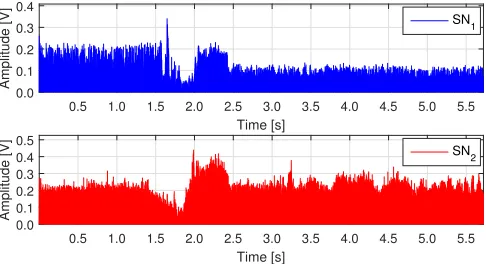
Fig. 9. Communication recorded from two different locations SN1and SN2.
following basic elements: “1” IFS, “2” DATA and “3” ACK. Accordingly, the hidden state St at time t is a discrete
real-valued random variable that can take values in the set
S={1,2,3}. This corresponds to capturing the channel from a single measurement point.
In this section, we are concerned with the case where multiple channel traces from the same source are concurrently monitored from different measurement points. This amounts to deploying multiple time-synchronized receivers (sniffers) and have them listening to the same transmitter. The rationale is that the channel realizations that they respectively see are likely to be uncorrelated. This can provide significant improvements to the detection performance. In Fig. 9, we show the same transmission captured by two different sniffers, labeled SN1 and SN2.
In this scenario, the observed channel samples in the data burst are modeled as a sequence of multi-dimensional, real-valued random variables, OOO1:T = (OOO1, . . . , OOOT), where
T is the data burst length. The observation vector associated with channel sample t,OOOt, is a probabilistic function of the
hidden stateSt. According to the Gaussian-observation model,
P(OOOt|St=i) =N(OOOt;µµµi,ΣΣΣi), whereµµµiandΣΣΣi respectively
specify the multi-dimensional mean and the diagonal covari-ance matrix of the random vectorOOOt, given that the hidden
state is i ∈ S. For all hidden states i ∈ S, we collect the parameter pairsbi= (µµµi,ΣΣΣi)through vectorbbb= [b1, . . . , b|S|], as for the one-dimensional case. For Baum’s re-estimation approach [29], we have:
µµµnewi =
PT
t=1γt(i)ooot PT
t=1γt(i)
ΣΣΣnewi =
PT
t=1γt(i)(ooot−µµµi)
T(ooot−µµµi)
PT t=1γt(i)
, (4)
where ooot is the realization of OOOt, ξt(i, j) and γt(i) are
computed using the Forward-Backward algorithm, see [30], [31], and(·)Tdenotes vector transpose. Here, we assume that
there is no correlation among the observed channel samples from multiple viewpoints, henceΣΣΣi is a diagonal covariance
matrix for i ∈ S. In the following, the sniffers are denoted by SNdim, wheredim = 1,2, . . .. Moreover, when the hidden
state isi∈ S, we refer to the element in positiondiminµµµias
µ(dim)i and to thedim-th diagonal element ofΣΣΣi as Σ (dim)
X. MM-WAVE TRACE GENERATOR
Need for the ground truth:a ground truth signal is necessary to precisely quantify the reconstruction performance of the one- and the multi-dimensional protocol analyzers. This would amount to acquire the actual protocol state that is associated with each sample inOOO1:T. In practice, this could be achieved
using a tool such as Wireshark on a monitor node. Unfor-tunately, state-of-the-art 802.11ad hardware is still unable to reliably provide such information to the higher layers. The protocol state sequence that is extracted by the radio is usually incomplete (some frames are missing), the states are shifted in time (with distorted inter-spaces) and often their order is also affected. The only metric that current devices can reliably provide are cumulative counters of packet types (see Section XI-A for further discussion and experimental results). To overcome this, we have developed a realistic mm-wave trace generator, with the goal of reproducing narrowband physical layer energy traces from one or multiple sniffers in a fast and accurate manner. This makes the evaluation of our diagnosis tool possible, providing quantitative results in a range of practical scenarios. The developed generator repro-duces typical IEEE 802.11ad data burst sequences, mimicking random fluctuations in the channel dynamics, variability in the number and duration of DATA and ACK frames, etc. These burst sequences are separated by beacon pairs (also affected by channel noise), whereas other control messages, appearing outside the data bursts, are not modeled as they are not involved in our performance assessment.
This tool has been instrumental in the fine tuning of the EDHMM model, as it allows for a precise control of the energy levels associated with transmissions from the source and channel noise. Next, we detail its structure, which is organized into macro- and micro-states. Macro-states describe different instances of the channel transmission setup, i.e., a specific combination of coding and modulation schemes, and we assume that macro-state transitions can only occur at the end of data bursts. Instead, micro-states track the duration of DATA and ACK frames within a data burst, for any given setup (macro-state). Each data burst starts with a beacon pair and the system remains in the same macro-state for the entire duration of the burst. Once in a data burst, the micro-state model returns the sequence of DATA and ACK frames.
Notation: the superscript (0) is used for the macro-model parameters. The macro-state takes values in the set M(0) = {1, . . . ,|M(0)|} and evolves according to the transition
ma-trix TTT(0), with steady state distribution πππ(0). If the current macro-state is M ∈ M(0), the micro-state m takes values in
the set M(M) ={1, . . . ,|M(M)|} and evolves according to
the transition matrixTTT(M), with steady state distributionπππ(M). The macro-model:macro-states capture different instances of the channel transmission setup, i.e., |M(0)| different
combi-nations of coding and modulation schemes. For each macro-state M ∈ M(0), the following statistics are specified: (i) the
PMF P(d(M)IDLE) of the idle time d(M)IDLE between subsequent packets, (ii) the joint PMF P(d(M)DATA, d(M)ACK) of DATA and ACK durations, respectively termedd(MDATA) andd(M)ACK, where the ACK is the frame following the DATA one in the hidden
state sequence (s1, . . . , sTn), and (iii) the PMF P(d (M) burst)of
the duration of data bursts, d(Mburst). The following remarks are in order:
• We have experimentally verified thatP(d(M)DATA, d(M)ACK)6=
P(d(M)DATA)P(d(M)ACK), which means that there exists some correlation between the marginal random variables mod-eling DATA and ACK durations. This is due to frame aggregation, which results in block acknowledgments. Such acknowledgments are longer than the regular ac-knowledgments used for shorter, non-aggregated frames. • Stationary channel traces are utilized to obtain the dura-tion statistics of idle times, DATA packets and ACKs. As done for the online estimation via time-adaptive EDHMM, upon obtainingΘ(n)EDHMM for the current data burst o(n)1:T
n, the corresponding hidden state sequence
(s1, . . . , sTn) is reconstructed using the Viterbi
algo-rithm with samples o(n)1:T
n = (o1, . . . , oTn). From these
estimates, duration statistics for the elements in the set
S={1,2,3} and for the data burst itself are obtained. • Transitions between macro-states occur at the end of each
data burst according to the transition matrixTTT(0). This
makes it possible to probabilistically model variations in the protocol behavior due to, e.g., soft link blockages (e.g., waiving a hand in the boresight of the antenna) or to modifications of the received energy due to a change in the orientation of the device.
The micro-model: consider a data burst in any macro-state
M. Within this data burst, a sequence of DATA-ACK frames is exchanged, and the duration of such packets is controlled by the micro-model. Specifically, the domain of the PMF
P(d(M)DATA, d(M)ACK) is clustered into |M(M)| rectangular
sub-domains through the Elbow method, which is a clustering technique to automatically determine the number of clusters
K [49]. We run this clustering algorithm twice: for the dimension associated with {d(MDATA) } and for that associated with{d(MACK)}, obtainingKDATA(M) andKACK(M) clusters for DATA and ACK frames, respectively. This leads to |M(M)|
rect-angular subdomains with |M(M)|=K(M)
DATA×K
(M) ACK. Each
of such domains m ∈ M(M) defines a micro-state with
conditional PMF P(d(MDATA) , d(MACK)|m), representing the joint distribution of DATA and ACK durations within that region (conditioned on the model being in region m). Transitions between micro-states occur according to the transition matrix
TTT(M), which is estimated from empirical data. The steady-state
probability vectorπππ(M)is obtained through numerical
Algorithm 1 Pseudo-code of the mm-wave trace generator 1: M =pick(πππ(0)); // pick macro-state
2: m=pick(πππ(M)); // pick micro-state 3: Set`= 0;˜yyy(dim)=empty vector(); 4: while` < L do
5: T =pick(P(d(Mburst))); 6: fordim = 1 to2do
7: yyy˜(dim)=concatenate(˜yyy(dim), tmptmptmp(dim)); 8: Sett= 0;ooo(dim)=empty vector();
9: whilet < T do
10: d1=pick(P(d (M) IDLE));
11: (d2, d3) =pick(P(d (M) DATA, d
(M) ACK)|m);
12: ooo0 =create frames(d1, d2, d3); 13: ooo(dim)=concatenate(ooo(dim), ooo0); 14: // Change current micro-state? 15: m=next state(TTT(M), m);
16: t=length(ooo(dim));
17: end while
18: yyy˜(dim)=concatenate(˜yyy(dim), ooo(dim));
19: end for
20: Mprev=M;
21: // Change current macro-state? 22: M =next state(TTT(0), M); 23: if M 6=Mprev then
24: // resample from steady-state distribution 25: m=pick(πππ(M));
26: end if
27: `=length(˜yyy(dim)); 28: end while
see line 6. Each burst starts with a beacon pair, denoted by
tmp tmp
tmp(dim), which is a noisy version of the template used by the
template matching algorithm of Section VI. The beacons are concatenated to the output sequenceyy˜y(dim) in line 7, and the noisy data burst is created through the “while” cycle starting from line 9. Durations of DATA (d2), ACK (d3) frames and
of the IDLE time between them (d1) are respectively sampled from the PMFs P(d(MDATA) , dACK(M)|m)and P(d(M)IDLE). A noisy sequence composed of DATA (d2 samples), IDLE (d1 sam-ples), ACK (d3samples) and IDLE (d1 samples) is generated
through the “create frames()” function of line 12. The so obtained output samplesooo0 (of length2d1+d2+d3 samples) is then appended to the current sequence ooo(dim) (line 13). When the while cycle ends,ooo(dim) contains the noisy samples
associated with the new data burst. The noisy samples in the sequence, which are associated with hidden statei∈ {1,2,3}
(respectively IDLE, DATA and ACK), are computed as (ad-ditive Gaussian noise):µ(dim)i +
q
Σ(dim)i randn(1, di), where
“randn(1, di)” denotes a random vector ofdi elements, with Gaussian distributed entries N(0,1). Although not explicitly indicated, the sequence of hidden states is saved along with the noisy version y˜yy(dim) and used as ground truth for the performance evaluation of Section XI-B.
We now discuss some example results for the case of two macro-states. M = 1: distance TX-RX 1.5 m, MCS 11. M = 2: distance TX-RX 2.5 m, MCS 10. Empirical
0 50 100 150 200 250
d(1)DATA 0
100 200 300 400
d
(1
,
2
)
A
C
K
partition for macro-state 1
0 50 100 150 200 250
d(2)DATA partition for macro-state 2
Fig. 10. Empirical measurements(d(MDATA) , d(MACK)) for two marco-states. Rectangular regions are obtained using the Elbow method. Values in the axes are expressed in number of channel samples (the sampling frequency isTs= 0.1µs).
0 0.5 1 1.5 2
Time [ms] 0
0.01 0.02 0.03 0.04
PMF
burst length for macro-state 1
0.5 1 1.5 2
Time [ms] burst length for macro-state 2
Fig. 11. PMF of the burst lengthP(d(M)burst)for macro-models 1 and 2.
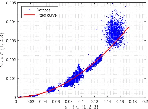
(d(MDATA) , d(MACK)) pairs are shown in Fig. 10 for M ∈ {1,2}, along with the rectangular regions obtained using the Elbow clustering algorithm. We observe that the duration statistics are more spread in model 1 with respect to macro-model 2, meaning less data aggregation. Also, the length of the data burst is shorter in macro-model 1, see Fig. 11. For each macro-state M, the domain (d(MDATA) , d(MACK))is split into clusters using the Elbow method: the number of clus-ters is greater in macro-model 1, i.e., KDATA(1) =KACK(1) = 6 and KDATA(2) =KACK(2) = 3.6 Fig. 12 shows empirical points (µ(dim)i ,Σ(dim)i )for different channel setups. In this plot, we do not distinguish between statesi∈ {1,2,3}, as our purpose is to establish a suitable relation between mean (µ) and variance (Σ) of the received energy levels, and the difference in the received energy levels captured by the sniffers depends on the relative position of the sniffers with respect to the communicating devices. These empirical points were fitted through the following curve (the red solid curve in the plot):
Σi=c1µci2, i∈ {1,2,3}, (5)
with c1 = 0.105 and c2 = 1.905. The coefficients c1 and c2 were found through a linear regression in the logarith-mic domain, i.e., we fit the dataset taking into account the
6The number of clusters is chosen such that the percentage of variance
0 0.02 0.04 0.06 0.08 0.1 0.12 0.14 0.16 0.18 0.2
µi,i∈ {1,2,3}
0 0.001 0.002 0.003 0.004 0.005
Σi
,
i
∈
{
1
,
2
,
3
}
Dataset
Fitted curve
Fig. 12. Gaussian observation model: empirical values and fitting curve for mean (µ) and variance (Σ) of the received energy levels associated with IDLE periods, DATA and ACK frames.
logarithmic counterpart of the datapoints and minimize the total residual error, obtaining an excellent goodness of fit (R2= 0.9595, whereR2 is the coefficient of determination).
The linear relationship in the logarithmic domain of Eq. (5), that we obtained empirically, is also confirmed by previous analytical work on RSS localization, see, e.g., [50], [51].
As a final consideration, we note that the average energy levelsµi and their variancesΣiremain constant for the entire
duration of the data bursts, which is a key assumption in the developed EDHMM algorithm (see assumption A3, in Section V). In the numerical results, we assess the performance of our algorithms when assumption A3 is no longer verified, i.e., when µi and Σi do change within a DATA burst. This
is achieved through anadditivesinusoidal noise of frequency
f, which is added to the generated energy traces, by tuningf
and the noise amplitude.
XI. PERFORMANCE RESULTS
Next, we present some selected performance results. Exper-imental results are discussed in Section XI-A, considering sin-gle and multiple time-synchronized sniffers. The performance of our tool is further quantified in Section XI-B, using the mm-wave trace generator of Section X.
A. Evaluation with experimental data
We consider the setup in Section VI. First, we validate our machine learning framework in controlled scenarios. Next, we study the behavior of indoor links during regular operation to check how our framework can identify and characterize effects such as beam misalignment.
Validation in controlled scenarios: Fig. 13 shows a trace decoding example for our diagnosis tool. In the upper part of the figure, we show the raw trace as captured by the Sivers IMA converter. The two initial frames are beacons that indicate the start of a data burst. After that, we observe a sequence of data and acknowledgment frames (c.f. Fig. 1). The lower part of the figure shows that our framework can correctly identify all frames in the trace. We observe that the
250 500 750 1000 1250 1500
Sample number 0
0.1 0.2 0.3
Amplitude [V]
250 500 750 1000 1250 1500
Sample number 1
2 3 4
State number
HMM EDHMM
Fig. 13. Trace decoding example for our machine learning framework.
framework successfully classifies data packets, acknowledg-ments, beacons, and inter-frame spacing. Moreover, Fig. 13 also demonstrates the need for our EDHMM approach. The HMM method wrongly classifies many of the samples—within a data or acknowledgment frame, it often fluctuates between states. In contrast, the EDHMM classifies all samples correctly, even in case of varying data packet lengths.
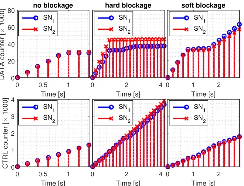
In addition to the visual inspection in Fig. 13, we validate our framework using two approaches. First, we compare the number of data packets that our tool identifies with the number of packets that the driver of our 60 GHz device reports. For the case without blockage in Fig. 14, the driver reports31960 sent packets at the end of the trace. This matches the data packet counter in our results. Second, we record the same data exchange using two independent sniffers SN1 and SN2,
and process the resulting traces using our framework. For no blockage, Fig. 14 shows that both sniffers count the same number of both data and control packets. This again validates that our framework is correctly decoding the trace. For data packets, the counter stabilizes at one second at which point we stop the data transmission. Still, the control packet counter increases steadily because the devices continue to exchange control packets even if no data transmission is taking place.
Fig. 14 also depicts similar measurements for two blockage cases. The first is a “hard blockage”, i.e., crossing the link and thus interrupting it completely for a few milliseconds. The second is a “soft blockage”, which refers to partial blockage such as waiving a hand in the boresight of the antenna. These blockages cause a drop in the energy levels captured by the two independent sniffers SN1 and SN2, which actually perceive a
different number of both data and control packets due to the different relative positions of the sniffers with respect to the mm-wave link.
no blockage
0 0.5 1
Time [s] 0
20 40 60 80
DATA counter [
×
1000]
SN1
SN2
hard blockage
0 2 4
Time [s] SN1
SN2
soft blockage
0 1 2
Time [s] SN1
SN2
0 0.5 1
Time [s] 0
1 2 3 4
CTRL counter [
×
1000]
SN1
SN 2
0 2 4
Time [s] SN1
SN 2
0 1 2
Time [s] SN1
SN 2
Fig. 14. Number of data and control packets identified by our tool. We show the results for two sniffers SN1and SN2placed at different locations.
result in suboptimal performance, and which our framework can identify. The protocol used by our 60 GHz test devices defines that the maximum burst length is two milliseconds and the maximum aggregated packet length is20microseconds [6]. Since we perform this experiment with full transmission buffer at the nodes, the burst and packet lengths should match the maximum values.
For the different measurements, the link distance is main-tained to be equal to3meters, while the rotation of the nodes varies, resulting in changes in the MCS and frame duration. Specifically, for Link 3 the antennas of the devices are facing one another, whereas for Link 1 and 2 they are not. While the MCS of Link 1 and 2 are the same, for Link 1 in Fig. 15 we observe smaller packet durations. To reduce the packet error rate when the link quality is worse, the MAC reduces the level of aggregation, i.e., the MAC layer aggregates fewer data packets than the maximum into a single MAC packet. Indeed, our framework also reveals that the trace energy level differs compared to Link 2, which suggests antenna misalignment. We omit the energy trace level in the interest of space but the device driver reveals that both Links 1 and 2 operate otherwise identically in terms of MCS and traffic load. In other words, our framework successfully identifies the suboptimal device orientation for Link 1. Fig. 15 shows that Link 3 performs even better in terms of packet length. Again, the device driver confirms this insight since Link 3 uses a more robust MCS than Link 2. Thus, Link 3 is more likely to succeed when transmitting longer packets.
External disturbance: regarding external disturbances, we focus on the case of link blockage. Our tool is able to identify and classify such blockage. This provides means for network operators to determine how often blockage actually occurs for a certain mm-wave link during a certain time-frame, for instance, a day.
Identifying blockage is challenging because it may block the LOS path to the sniffer, too. To prevent this, our framework can record and compare the channel activity from two or more sniffers at different locations, as shown in Fig. 16. We
burst length
0.5 1 1.5 2
Time [ms]
Link 1: MCS = 11, BPA
Link 2: MCS = 11, BPB
Link 3: MCS = 8, BP B
DATA length
5 10 15 20 25
Time [µs] 0
0.2 0.4 0.6 0.8 1
ECDF
Link 1: MCS = 11, BPA
Link 2: MCS = 11, BPB
Link 3: MCS = 8, BP B
Fig. 15. CDF of packet and burst lengths for three links deployed in the same environment but with varying performance. “BP” stands for beampattern.
1.929 1.930 1.931 1.932 1.933
Time [s] 0.0
0.1
Amplitude [V]
SN1
1.929 1.930 1.931 1.932 1.933
Time [s] 0.0
0.1 0.2
Amplitude [V]
SN2
Fig. 16. Blockage recorded from two different locations SN1and SN2. The
figure shows a fraction of the blockage, i.e., the blockage affects all samples.
observe that while sniffer SN1 barely receives any of the
activity prior to second1.93, SN2 is able to receive all frames
during the blockage. This allows our framework to obtain a much more complete view of the activity on the channel. Based on this information, we automatically identify beam refinement (BR) sequences. Such sequences are rare in static scenarios but are likely to occur if the link is impaired. Fig. 17 depicts a segment of the trace in Fig. 16, overlapped with the locations at which our framework identifies BR sequences. We observe that the BRs identified by both sniffers match but that not all sniffers capture all sequences due to the blockage. This highlights again the benefit of being able to analyze the network behavior from multiple viewpoints. Moreover, Fig. 16 depicts a soft blockage. Thus, the connection does not break and the device continuously adapts its beampattern, resulting in a large number of BRs. In contrast, hard blockage results in less BRs since the transmitter and the receiver cannot communicate during the blockage. As per our measurements, the average number of BRs per trace for no blockage, hard blockage, and soft blockage is 0 BRs/trace, 0.42 BRs/trace, and 4.02 BRs/trace, respectively. The difference in terms of BR frequency allows our diagnosis tool to classify blockage. This is highly valuable to determine why a mm-wave link is performing poorly.