waveformlidar: An R package for waveform LiDAR processing and
1analysis
2Tan Zhou1,2*, Sorin Popescu2
3
1 Colaberry Inc., 200 Portland St, Boston, MA 02114, USA: [email protected] 4
2 LiDAR Applications for the Study of Ecosystems with Remote Sensing (LASERS) 5
Laboratory, Department of Ecosystem Science and Management, Texas A&M University, 6
College Station, TX 77450, USA; 7
Abstract
8
A wealth of Full Waveform (FW) LiDAR data are available to the public from different sources, 9
which is poised to boost the extensive application of FW LiDAR data. However, we lack a handy 10
and open source tool that can be used by potential users for processing and analyzing FW LiDAR 11
data. To this end, we introduce waveformlidar, an R package dedicated to FW LiDAR processing, 12
analysis and visualization as a solution to the constraint. Specifically, this package provides several 13
commonly used waveform processing methods such as Gaussian, adaptive Gaussian and Weibull 14
decompositions, and deconvolution approaches (Gold and Richard-Lucy (RL)) with users’ 15
customized settings. In addition, we also developed functions to derive commonly used waveform 16
metrics for characterizing vegetation structure. Moreover, a new way to directly visualize FW 17
LiDAR data is developed through converting waveforms into points to form the Hyper Point cloud 18
(HPC), which can be easily adopted and subsequently analyzed with existing discrete-return 19
LiDAR processing tools such as LAStools and FUSION. Basic explorations of the HPC such as 20
3D voxelization of the HPC and conversion from original waveforms to composite waveforms are 21
also available in this package. All of these functions are developed based on small-footprint FW 22
LiDAR data, but they can be easily transplanted to the large footprint FW LiDAR data such as 23
Geoscience Laser Altimeter System (GLAS) and Global Ecosystem Dynamics Investigation 24
(GEDI) data analysis. It is anticipated that these functions will facilitate the widespread use of FW 25
LiDAR and be beneficial for better estimating biomass and characterizing vegetation structure at 26
various scales. The package and code examples can be found at 27
https://github.com/tankwin08/waveformlidar. 28
1 Introduction
29
The advent of Full Waveform (FW) LiDAR data including airborne and spaceborne have enabled 30
new opportunities for vegetation structure characterization at a range of scales [1-5]. Unlike 31
Discrete-return (DR) LiDAR data which only store the signal whose intensity higher than the 32
system-defined threshold, FW LiDAR data can store the entire echo scattered from illuminated 33
objects with different temporal resolutions [1,6]. This advantage provides more information about 34
the objects the pulse interacts with and gives users more flexibility to interpret information inherent 35
in waveforms [7]. 36
Multiple approaches such as the Gaussian decomposition and deconvolution have been developed 37
to interpret information from waveforms [6,8,9]. However, complicated processing steps and 38
algorithms hinder the widespread use of FW LiDAR data. To tackle these challenges, our package 39
waveformlidar proposed several commonly used approaches and functions to conduct waveform 40
processing and analysis such as Gaussian decomposition and deconvolution. These approaches 41
have been successfully applied to extract physical attributes of vegetation such as canopy height, 42
stem volume, aboveground biomass and tree species from LiDAR waveforms [2,3,10]. With the aid 43
of the package, these approaches can be easily implemented in the R platform and further relieve 44
users’ concerns on complicated FW processing steps. 45
Additionally, currently available tools are mainly oriented for processing DR LiDAR data. There 46
is a lack of handy tools that work with FW LiDAR data which precludes potential users to explore 47
the usefulness of FW LiDAR data. Therefore, we developed functions to derive commonly used 48
waveform metrics such as front slope and waveform distance. These waveform metrics are 49
different from the metrics derived from waveform decomposition in terms of the information they 50
contained. Thus, they can be complementary to metrics obtained from decomposition, which 51
enable users to make the most use of the waveform information contained. 52
Lastly, the package also proposed a new method to convert waveforms into point clouds with hyper 53
point density (Hyper Point Cloud, HPC) and composite waveforms after implementing waveform 54
voxelization steps. The HPC is an alternative product of FW LiDAR data, which not only can 55
preserve information embedded in original waveforms, also offer users a convenient way to 56
visualize and decode information with existing LiDAR processing tools such as LAStools [11] and 57
FUSION [12]. However, not every waveform signal is useful for real-world applications. To 58
explore the HPC’s potential usefulness, this package also provides functions to explore the HPC 59
in 2D and 3D spatial dimensions. Additionally, we also explore the methods to convert original 60
with intensities distributing at the vertical direction. We also conducted a comparison between 62
original waveforms and composite waveforms on the tree species identification and detailed 63
information can be found in Zhou et al. [13]. Notably, the storage and computation cost using the 64
composite waveforms is more expensive than original waveforms, which requires users to conduct 65
an assessment of the marginal benefits obtained from composite waveforms. 66
Overall, the purpose of this article is to provide an overview of the waveformlidar package and to 67
ensure the free availability and usability of methodologies including code or algorithms from our 68
previous scholarly publications. We first introduce an example of FW LiDAR data and 69
corresponding ancillary data such as outgoing pulse and system impulse data. Next, we begin to 70
briefly explain the main algorithms’ technical principles and the logic behind them. We end by 71
discussing the main functions such as decomposition, deconvolution and the HPC in the practical 72
use in the R platform. Full tutorials and reports to reproduce the results from these examples are 73
available in the supporting information from our website
74
(https://github.com/tankwin08/waveformlidar). 75
2 Example datasets
76
FW LiDAR data are available on the market with various formats. However, they are primarily 77
composed of two parts: a pulse part that keeps geo-reference locations derived from range 78
measurement between the laser sensor and the reference location, and a wave part which stores 79
digitized return energy starting from the reference location till the end of digitized samples [4]. To 80
mitigate the effect of format on the FW LiDAR data processing, we converted these files into CSV 81
format and then conducted the subsequent analysis. The waveform LiDAR datasets were 82
downloaded from National Ecological Observatory Network (NEON) data center 83
(http://www.neonscience.org/content/airborne-data). The example dataset used here is a subset 84
(500 waveforms) from the Harvard Forest, Massachusetts, USA. Each row represents one 85
waveform and each column represents a time bin. The temporal resolution of the time bin can be 86
1/2/4 nanosecond (ns), which is up to the data collecting system. In this case, the temporal 87
resolution is 1 ns with the vertical distance approximately 0.15m. 88
Overall, there are two major methods for waveform processing in this package. The first method 89
was direct decomposition (I), which only applied the Gaussian, adaptative Gaussian and Weibull 90
decomposition (II) method. More details of these two methods are elaborated in the Methods 92
section. Most of the functions in the waveformlidar package require waveform LiDAR data as the 93
input for obtaining useful information. However, the method II requires additional input data such 94
as corresponding outgoing pulse data, system response impulse and its corresponding outgoing 95
pulse to interpret information inherent in waveforms. Ideally, the system response pulse would be 96
measured in the lab using a hard target. Here, the system response impulse was a return pulse of a 97
single laser shot from a hard ground target with a mirror angle close to nadir [6]. Through 98
deconvolving the outgoing pulse corresponding to this system response pulse, we obtain a closer 99
system response pulse closer to the true system response pulse. With the aid of the system response 100
impulse and its corresponding outgoing pulse, the system response effect can be removed with the 101
deconvolution method. Generally, we can assume the system response pulse the data vendor 102
provided is the true system response pulse. In the Deconvolution section, we provided an example 103
to show the detailed deconvolution process. In addition, we also provided two example results 104
with the two different methods. In summary, we provided 8 datasets in this package and their 105
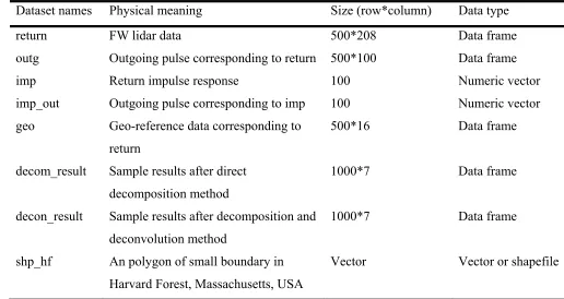
corresponding brief introduction as shown in Table 1. 106
Table 1. A summary of example data sets for waveformlidar package. 107
108
Dataset names Physical meaning Size (row*column) Data type
return FW lidar data 500*208 Data frame
outg Outgoing pulse corresponding to return 500*100 Data frame
imp Return impulse response 100 Numeric vector
imp_out Outgoing pulse corresponding to imp 100 Numeric vector
geo Geo-reference data corresponding to return
500*16 Data frame
decom_result Sample results after direct decomposition method
1000*7 Data frame
decon_result Sample results after decomposition and deconvolution method
1000*7 Data frame
shp_hf An polygon of small boundary in Harvard Forest, Massachusetts, USA
Vector Vector or shapefile
3 Methods and functions
110
3.1 Methods
111
3.1.1 Decomposition and deconvolution 112
The waveformlidar package provides two broad sets of methods including the deconvolution and 113
decomposition to interpret useful information from waveform LiDAR data. These two methods 114
are built on different assumptions. For the deconvolution, we assumed that the returning pulses of 115
the waveform were the product of interaction among outgoing pulses, atmospheric scattering, 116
system noise and reflecting surfaces. In other words, the return waveform can be expressed as the 117
convolution of the outgoing pulse, impulse response (atmospheric scattering, system noise, etc.) 118
and effective target cross section [6,7] (Eq. (1)). 119
𝑃 𝑡 ∑ 𝑃 𝑡 ∗ 𝜏 𝑡 ∗ 𝛿 𝑡 (1)
120
where 𝑃 𝑡 is the received laser power, 𝑃 𝑡 is the emitted laser power, τ t is the receiver 121
impulse function, D is the aperture diameter of the receiver optics, λ is the wavelength, R is the 122
range from the LiDAR system to the target and 𝛿 𝑡 is the effective target cross section. 123
Thus, the deconvolution is an algorithm-based process that is to reverse the effect of convolution 124
on the recorded signals, and the decomposition is a process which can provide estimates of the 125
location and properties of objects along the pulse [7]. In this package, two deconvolution methods 126
including the Gold and Richardson-Lucy (RL) are available for conducting the deconvolution. The 127
detailed description of these algorithms can be found in [6]. 128
For the decomposition, both the outgoing pulse and the return pulse are nearly following some 129
probability distribution such as Gaussian distribution in terms of shape. Thus, the information 130
inherent in waveform can be extracted through fitting waveforms with a mixture of models with 131
the specific distribution or waveform components. By interpreting these models’ parameters or 132
waveform components, the targets such as vegetation and ground interacting with outgoing pulse 133
along the path can be characterized. 134
In this package, three representative models such as the Gaussian (Eq. 2), Adaptative Gaussian 135
(Eq. 3) and Weibull (Eq. 4) models [4,9] were available to interpret information from waveforms. 136
The Gaussian model is the most frequently used model for waveform decomposition. In general, 137
the outgoing pulse is assumed to be Gaussian shape, as well as the effective target cross-section 138
return waveform also follows the Gaussian distribution in the ideal condition. Therefore, the return 140
waveform can be fitted with a mixture of Gaussian models. 141
𝑓 𝑥 ∑ 𝐴 exp (2)
142
where n is the number of Gaussian components, 𝐴 is the amplitude of ith waveform component,
143
𝛿 is the standard deviation of ith waveform component, and 𝑢 is the time location of ith waveform
144
component. 145
The Adaptive Gaussian model has the form of Eq. (3) which can minimize the residual of the 146
model by introducing another variable which is also known as rate parameter (λ). 147
𝑓 𝑥, 𝜃 ∑ 𝐴 exp (3)
148
The Weibull model (Eq. 4) was introduced since it enables us to simulate either symmetric or 149
asymmetric peaks with four unknown parameters (8-3). 150
𝑓 𝑥, 𝜃 ∑ 𝐴 exp (4)
151
where Ai is the amplitude, k (> 0) is the shape parameter that controls the behavior or the shape of
152
the distribution, and δi (> 0) is the scale parameter that controls the spread of the distribution. The
153
shape parameter can capture the asymmetry or skewness of the waveforms that overcomes the 154
disadvantage of the Gaussian function, which is only suitable for symmetric distributions. ui is a
155
location parameter in the Weibull model. 156
3.1.2 Hyper point cloud 157
The methods mentioned in Section 3.1.1 are mainly intended to convert part of waveform signals 158
into points to form DR-like point clouds with additional information such as amplitude (A) and 159
echo width (𝛿). However, intensity information embedded in waveforms, which is the most 160
conspicuous advantage of FW LiDAR data, is still insufficiently studied. Moreover, the 161
decomposition or deconvolution method requires users to have a deep understanding of 162
complicated waveform processing methods and precludes practitioners’ willingness to explore FW 163
LiDAR data’s potential. To overcome these technical barriers and make the most use of waveform 164
information, we proposed a new concept named Hyper Point Cloud (HPC) to directly convert all 165
product also renders us a direct way to visualize the FW LiDAR data with existing tools or software 167
mainly oriented toward DR LiDAR data processing. 168
Beyond the concept of the HPC, we also developed some algorithms to explore potential 169
applications of the HPC. For example, the waveformgrid and waveformvoxel are primarily meant 170
to generalize information at the 2D and 3D spatial scale from the HPC. The logic of these two is 171
to project waveform information into 2D grid cells or voxels to obtain high-level information of 172
objects according to the user defined resolution. Furthermore, we also developed an algorithm 173
(rawtocomposite) to generate composite waveforms with waveform signals are vertical 174
distributed. It is anticipated that this product can reduce the impact of tilt angle on the vegetation 175
characterization in the vertical direction. 176
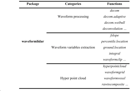
To get a better overview of our package, we summarized the major functions in Table 2. 177
Table 2. Summary of major functions of waveformlidar package 178
Package Categories Functions
Waveform processing
decom decom.adaptive
decom.weibull deconvolution …
waveformlidar
Waveform variables extraction
fslope percentile.location
ground.location integral waveformclip …
Hyper point cloud
hyperpointcloud waveformgrid waveformvoxel rawtocomposite …
179
3.2 Functions with examples
180
As shown in Table 2, the waveformlidar package consists of three major components: waveform 181
processing, waveform variable extraction, and HPC generation and its potential applications. The 182
Installation 184
To install the latest release version from CRAN, type install.packages("waveformlidar")
185
within R. The current developmental version can be downloaded from GitHub via: 186
if (!require("devtools")) {
187
install.packages("devtools")
188
}
189
devtools::install_github("tankwin08/waveformlidar", dependencies = TRUE)
190
3.2.1 Preprocessing 191
The waveform processing involves a series of preprocessing steps such as noise detection, 192
smoothing and radiometric calibration. In this package, we provide some options in several 193
functions to conduct the preprocessing steps. 194
Different data sources may store data in different radiometric resolution or start at different 195
baseline values. For instance, the NEON FW LiDAR data are 16 bits, and the baseline value of the 196
waveform is about 200. To optimize subsequent analysis, we applied the minimum subtraction for 197
each waveform to ensure that the signal intensity starts at 1. 198
Before conducting waveform processing with the decomposition or deconvolution methods, 199
several functions are also available to obtain general information about the waveform echoes. For 200
example, the lpeak function can be used to identify the peak location in each waveform with TRUE 201
and FALSE; the npeaks function is to identify the number of waveform components (n) of models 202
being used. Another important function is the gennls, which is used to generate the non-linear 203
Gaussian model formula for each waveform based on the number of waveform components and 204
the probability distribution model the users chose. Moreover, this function also gives the model 205
appropriate initiated estimates for parameters such as 𝐴 , 𝑢 and 𝛿 to ensure the successful 206
solutions of waveform fitting. For example, if one waveform was identified with the three 207
waveform components and the corresponding initialized parameters are given as follows: 208
library(waveformlidar)
209
A<-c(76,56,80); u<-c(29,40,67); sig<-c(4,3,2.5)
210
The Gaussian model can be generated automatically with these known parameters. 211
fg<-gennls(A,u,sig)
212 213
fg returns two parts: fg$formula gives the formula of the Gaussian model, and fg$start provides 214
the initiated values for each parameter based on known values. 215
The models suitable for the waveform fitting are the non-linear models that generally suffer from 216
used for fitting one waveform. Thus, this package also provides another two representative models 218
such as the Adaptative Gaussian (agennls) and Weibull functions (wgennls) to generate formulas 219
and initiate parameters for the model fitting. These two functions both have four parameters which 220
require us to give four vectors to initiate parameter estimates. The only difference between the 221
Gaussian function and Adaptive Gaussian function is the rate parameter r. When r = 2, the adaptive 222
Gaussian function becomes the Gaussian function. For example, the Adaptive Gaussian model 223
given the three waveform components can be generated as follows: 224
A<-c(76,56,80); u<-c(29,40,67); sig<-c(4,3,2.5); r<-c(2,2,2)
225
afg<- agennls(A,u,sig,r)
226
afg$formula
227
The Weibull function also has four parameters, but their physical meanings are different from the 228
Gaussian and adaptive Gaussian functions. The detailed description of these parameters can be 229
found in the study of Zhou and Popescu [4]. 230
In addition to using models to decompose waveforms, a function named peakfind is also available 231
to roughly estimate the parameters based on waveform shapes. 232
rough_estimates<- peakfind(wf[182,])
233 234
In the matrix of rough_estimates, the number of rows represents the number of waveform 235
components, and the columns corresponds to the index number of the waveform, the estimated 236
amplitude, time location(s) and echo width(s) of the corresponding waveform component(s). As 237
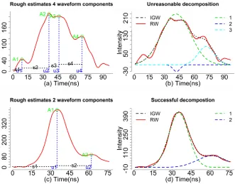
shown in Fig. 2 (a), the green circles (I) represent the estimated amplitude, the vertical blue dash 238
lines (m) represent the corresponding time locations and the horizontal dash lines (s) represent the 239
estimated echo widths. With the default, we can obtain four sets of parameters for four waveform 240
components (peaks). In fact, the first peak parameters may be caused by noise. 241
Actually, most of the waveforms are mixed with noise as we have shown in Fig. 2(b). There is a 242
difference between the ideal Gaussian waveform (IGW, black dash line, generated from a mixture 243
of Gaussian functions) and the raw waveform (RW, red). Consequently, some unreasonable peaks 244
maybe detected when the RWs mixed with a high level of noise. To obtain more reasonable results, 245
we need to conduct some preprocessing steps such as smoothing and threshold filtering. For 246
example, we increased the threshold to 0.3 to achieve a more reasonable rough estimate 247
(rough_estimates1). 248
rough_estimates1<- peakfind (wf[182, ], thres = 0.3)
250
Fig. 2. (a). The rough estimates derived from the waveform with four waveform components using 251
the peakfind function. (b). Illustration of the ideal Gaussian distribution waveform (IGW, black 252
dash) vs. real waveform (RW, red) using the waveform of (a). (c) The rough estimates derived 253
from the waveform with two waveform components using the peakfind function. (b). Illustration 254
of the ideal Gaussian distribution waveform (IGW, black dash) vs. real waveform (RW, red) using 255
the waveform of (c). The number such as 1 2 or 3 represents the individual Gaussian component. 256
3.2.2 Decomposition 257
Similar to the peakfind function, our core function decom also had an option named thres to enable 258
users to specify the threshold (thres*maximum intensity of the given waveform) for selecting peaks 259
and determine the number of waveform components. Another two important arguments are smooth
260
and width which are used to determine if we applied mean filter and the width of mean filter to 261
reduce the negative effect of noise on the waveform decomposition. The default is to use the 262
smooth function with the width = 3. The width argument is valid only when the smooth = TRUE. 263
For an individual waveform, we can implement the following codes to obtain the decomposition 264
result using the smoothed waveform (r1) and the raw waveform (r2). 265
r1<- decom(wf[1,])
266
r2<- decom(wf[1,], smooth = FALSE)
Results of decomposition are stored in a list, which consists of three components: the first is the 268
index of waveform for tracking the results from each waveform; the second is the raw results with 269
all estimated parameters; the third one is to extract parameters from the second result such as 270
estimates and standard error of the estimates, which is mainly to prepare for calculating the point 271
cloud from the decomposition results. 272
Results of r1 and r2 showed almost the same parameter estimates using smoothed and raw 273
waveforms. However, the decomposition results using the raw waveform may not give you a 274
solution to the complex waveform data fitting with an amount of noise. For example, the 275
decomposition of r3 just returns NULL due to the waveform being extremely irregular or to the 276
user rendering inappropriate initiating parameters. However, the decomposition results can be 277
achieved through adjusting the thres option such as smooth options (r4). With the appropriate peak 278
filtering steps, the waveform components can be obtained, and we plotted the Gaussian 279
decomposition in Fig. 2(a) with three waveform components. A closer examination reveals that 280
results of r4 are not reasonable since the A2 is negative, and u1 and u2 are too close (Fig. 2(a)). 281
To indicate this result is not reasonable, the index will return NA and the summary of parameters 282
will return NULL. For those waveforms without giving reasonable solutions, there are multiple 283
ways that can be explored to tackle these challenges. For instance, you can fit the waveform with 284
an additional waveform component or assign larger width to smooth the waveform again. In 285
addition, using other models or functions such as the peakfind or adaptive.decom functions are 286
also potential solutions. 287
r3<- decom(wf[182,])
288
r4<- decom(wf[182,],smooth=TRUE, width=7)
289 290
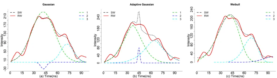
291
Fig. 3 An example of complex waveform with decomposition using the (a) Gaussian, (b) Adaptive 292
In addition, we also provided other similar models such as the adaptive Gaussian (decom.adaptive) 294
and Weibull functions (decom.weibull) (8-2) as alternatives to fit the waveforms. Compared to 295
decom, the decom.adaptive is able to fit the complex waveforms with default settings and is giving 296
us reasonable estimates. Of particular note, the adaptive Gaussian model may overfit the waveform 297
by adjusting the rate parameter (r) to minimize the model residual. Consequently, this may lead us 298
to mistakenly consider noise as waveform signal, and caution should be taken when we chose to 299
use this model. As shown in Fig. 3(b), three waveform components can be obtained using the 300
adaptive Gaussian models (r5) while the mixture of adaptive Gaussian function (black dash line) 301
is not consistent with the RW with obvious mismatch around time location 44 ns. 302
r5<-decom.adaptive(wf[182,])
303 304
As shown in Fig. 3(c), the decom.weibull function is also capable of fitting waveforms with three 305
waveform components using four parameters, but how to transform these parameters into a 306
meaningful product is still an open question. The four parameters of the decom.weibull have 307
different physical meanings compared to the decom and decom.adaptive functions. For the 308
decom.weibull, the A is the scaling factor which is related to the amplitude, u is the location 309
parameter, is the scale parameter and k is the shape parameter. Here, the scale parameter captured 310
the possible cross section information to some extent which may be used for generating point 311
clouds with additional steps. However, more efforts are still required to figure out how to transform 312
these parameters into meaningful products for waveform LiDAR, since the Weibull function is 313
originally designed for processing Synthetic Aperture Radar (SAR). 314
r6<-decom.weibull(wf[182,])
315
To demonstrate the efficiency of the algorithms and deal with large dataset, the apply function was 316
adopted. We explored this core function on a small dataset which contained 500 waveforms as 317
follows: 318
dr3<-apply(wf,1, decom.adaptive)
319
rfit3<-do.call("rbind",lapply(dr3,"[[",1)) ## to collect index information
320
ga3<-do.call("rbind",lapply(dr3,"[[",2)) ##to collect original results
321
pa3<-do.call("rbind",lapply(dr3,"[[",3)) #to collect estimated parameters for subsequent analysis
322
3.2.3 Deconvolution 323
Compared to the decomposition, the deconvolution requires more input data and additional 324
processing steps. Generally, we should have three kinds of data as the input for the deconvolution: 325
(SIR). The RW and OUT are directly provided by the vendor. Ideally, the SIR is obtained through 327
the calibration process in the lab before the waveform data are collected. In our case, NEON 328
provided a return impulse response (RIR) which can be assumed as a prototype SIR. This system 329
impulse was obtained through a return pulse of single laser shot from a hard ground target with a 330
mirror angle close to nadir. Meanwhile, NEON also provided the corresponding outgoing pulse of 331
this return impulse response (RIR_OUT). The “true” system impulse response can be obtained by 332
deconvolving the RIR_OUT. 333
In this package, we provide two options for users to deal with the system impulse response (SIR). 334
One is directly to assume the RIR as the SIR by assigning imp = RIR. Another is to obtain the SIR 335
through deconvolving the OUT_RIR. In the function, the “true” SIR can be achieved by assigning 336
imp = RIR and imp_out = OUT_RIR. 337
Two algorithms including the RL and Gold algorithms are available for the deconvolution. There 338
are three main parameters for the deconvolution algorithms: (1) iterations: number of iterations 339
between boosting operations; (2) repetitions: the number of repetitions of boosting operations, 340
which must be greater or equal to one; the total number of iterations is repetitions*iteration; and 341
(3) boosting coefficient/exponent: the exponentiation of iterated value. These parameters will be 342
valid only if repetition is greater than one and its recommended range is [1, 2]. Our experiments 343
showed that the boosting had less impact on the deconvolution results than the other two 344
parameters. The value of 1.8 was assigned for the default boosting coefficients. The number of 345
iterations and repetitions were critical to the performance of the deconvolution, which requires us 346
to conduct the optimization process. One way of conducting the optimization process had been 347
described in our previous study [6]. Moreover, the complexity of the waveforms generally required 348
larger number of iterations and repetitions, which spurred us to add two arguments (large_paras
349
and small_paras) for assigning suitable deconvolution parameters based on the number of 350
waveform components (nwc). The np is an integer as the threshold parameter for determining 351
using the large_paras (nwc > a anp) or small_paras (nwc <= np). For each argument, there are six 352
parameters including the iterations, repetitions and boost parameters for deconvolving the SIR and 353
the OUT. 354
data(return)
355
data(outg)
356
data(imp) ##The impulse function is generally one for the whole study area
357
data(imp_out)
re<-return[1,]
359
out<-outg[1,]
360
imp<-imp
361
imp_out<-imp_out
362
### option1: to obtain the true system impluse response using the return impluse repsonse (imp)
363
and corresponding outgoing pulse (imp_out)
364
gold0<-deconvolution(re = re,out = out,imp = imp,imp_out = imp_out)
365
rl0<-deconvolution(re = re,out = out,imp = imp,imp_out = imp_out,method = "RL")
366
###option2: assume the return impluse repsonse RIP is the system impulse reponse (SIR)
367
gold1<-deconvolution(re = re,out = out,imp = imp)
368
rl1<-deconvolution(re = re,out = out,imp = imp,method="RL",small_paras =
369
c(30,2,1.5,30,2,2))
370 371
After obtaining the deconvolution results, we can employ the peakfind, decom or decom.adaptive
372
functions to estimate the possible objects corresponding time locations and other related 373
parameters. The time location information will be used for the subsequent geolocation 374
transformation to generate the waveform-based point cloud. Other parameters can be appended to 375
the point cloud and provide additional information for vegetation characterization. 376
To exemplify differences of our waveform processing methods, we selected three waveform 377
examples to demonstrate results of decomposition and deconvolution methods in Fig. 4. The 378
detailed description of these methods has been reported in Zhou et al. [6]. 379
Fig. 4. Comparisons of the decomposition results with the direct decomposition approach, RL 381
approach and Gold approach for three sample pulses (a, b, c). The solid black line is the original 382
waveform. The colored dash lines are Gaussian components after decomposition [6]. 383
3.2.4 Geolocation transformation 384
This function is primarily used to transform waveforms into point clouds based on the 385
decomposition results and reference geolocation data. The reference geolocation data were 386
generally coming with the return waveforms and provided by the data vendor. Generally, reference 387
geolocation data include original x, y, z reference information (orix, oriy, oriz) and the position 388
change for x, y, z direction (dx, dy, dz) per time unit (ns). In addition, we also need to know the 389
first return reference bin location (refbin) for the decomposition results. For the deconvolution 390
results, the time of peak location for each outgoing pulse (outp) and the time of corresponding 391
reference bin location for the outgoing pulse (outref) is also needed. Detailed description of the 392
data and steps for calculation were given in Zhou et al. [14]. 393
Our package provided one function named geotransform to quickly integrate decomposition result 394
with reference geolocation data (geo) to generate points with relevant information. For the geo, we 395
need to assign specific names to each column, which were used to calculate the absolute position 396
of the time location in the waveform. To optimize the calculation process, we need to rename 397
column names of geo-reference data, which is critical to the successful implementation of the 398
function. 399
400
data(geo) ### the reference geolocation
401
##we need to assign names to geolocation datasets.
402
geoindex<- c(1:9,16)
403
colnames(geo)[geoindex]<-404
c("index","orix","oriy","oriz","dx","dy","dz","outref","refbin","outpeak")
405
decomre<-geotransform(decomp=rpars,geo)
406 407
Of particular note, the caution should be exercised in using this function. Because the geo-408
reference data format and their corresponding relationship with waveform data may vary for 409
different data vendors, which require users to explore the corresponding relationship for 410
subsequent calculation. 411
3.2.5 Waveform variables 412
In addition to classical methods such as the decomposition and deconvolution (Method 1), we also 413
waveform metrics or signatures from waveforms. Unlike the classical methods, waveform metrics 415
or signatures are directly obtained from waveforms instead of point cloud after decomposition. 416
Our package provides some functions to obtain waveform metrics or signatures such as the height 417
of median energy, front slope angle and the energy ratio between ground and vegetation from the 418
waveforms for serving purposes of the Method 2. For example, the fslope function can help 419
calculate the angle from waveform beginning to the first peak (front slope angle, FS), and the 420
distance from the waveform beginning to the first peak (ROUGH), both of which can be used to 421
differentiate the tree species in terms of crown structure. In addition, several intensity related 422
functions such as percentiles can easily get the intensity-based characteristic from the waveforms. 423
For example, we can calculate the intensity percentiles [0.45, 0.5, 0.55, …, 0.95] with 424
percentile.location function and obtain the relative time location of these percentiles. 425
data(return)
426
x<-return[182,]
427
qr<-seq(0.45,0.99,0.05)
428
re<- percentile.location(x)
429
With these time locations, we can calculate the relative height of these percentiles. We assumed 430
that the relative height is the height between the given location to the end of the waveform. To 431
calculate the relative height of these intensity percentiles, we need to assign top = FALSE to make 432
the intensity percentiles and the ground location index start at the end of the waveform. Another 433
factor we need to know for calculating the relative height is the temporal resolution of a waveform. 434
Here, our waveform was digitized with 1 ns temporal resolution which is approximately 0.15 m. 435
re1<-percentile.location(x,quan=qr,top=FALSE)
436
rh1<- (re1-ground.location(x,top = FALSE))*0.15
437
wd<- wavelen(x)*0.15
438
wgd<- (wavelen(x) - ground.location(x,top = FALSE))*0.15
439
num_peaks<- npeaks(x)
440
In this example, there is no negative value for rh1 since multiple waveform peaks are observed for 441
this waveform. The negative values of relative height represent these locations are below the 442
assumed ground level and caution should be exercised in real applications. Another important 443
function is to obtain the integral (the area under the waveform curve) of assumed vegetation and 444
assigning rescale = FALSE to conduct the integral calculation. But using the minimum intensity 446
(baseline) to conduct rescaling generally make more sense for generating integral related 447
parameters. 448
xx<-return[182,]
449
rr1<-integral(xx)
450
To demonstrate the waveform metrics derived from waveform, we plotted several of them in Fig. 451
5. Detailed description of these variables can be found in Zhou et al. [13]. Certainly, there are more 452
variables can be generated from the waveform based on the users’ purposes. 453
454
Fig.5. An example of waveform metrics such as the number of waveform peaks (orange triangle), 455
waveform distance (WD, red dash line), waveform distance from ground (WGD, dark green dash), 456
front slope (FS, green), height of half total energy(HOHE, red line), possible ground location (cyan 457
square), the integral of ground part (GI, gray area), the integral of vegetation part (VegI, blue area) 458
and the ratio of vegetation integral (RVegal) extracting from the waveform. 459
These functions were mainly oriented for one waveform. Some researchers or users may be more 460
interested in the waveforms within one specific region or given extent. The waveformclip function 461
of interest by specifying the geo-extent or a shapefile. It is worthy to note that the shapefile should 463
have the same projected coordinate system with the geo dataset. 464
data(geo)
465
colnames(geo)[2:9]<-c("x","y","z","dx","dy","dz","or","fr")
466
data(return)
467
waveform<-data.table(index=c(1:nrow(return)),return)
468
shp<-shp_hf
469
swre<-waveformclip(waveform,geo,shp)
470
swre1<-waveformclip(waveform, geo, geoextent=c(731126,731128,4712678,4712698))
471
Once a user has selected the waveforms within the region of interest (ROI), the functions used 472
above can be applied to these waveforms to obtain results up to users’ purpose. In addition, a user 473
also can combine theses waveform into one waveform and then process this waveform to obtain 474
the characteristic of objects within the ROI. 475
3.2.6 From waveforms to hyper point cloud 476
477
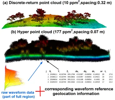
Fig. 6. (a) Discrete-return point cloud. (b) Illustration of the HPC generation concept using raw 478
To enrich existing waveform processing methods and reduce technical barriers of extracting useful 480
information from FW LiDAR data, we developed a new way to process FW LiDAR data by 481
converting all waveform intensities into points to form a very large point cloud dataset. The 482
concept of this method is illustrated in Fig. 6 by combing raw waveforms with corresponding 483
reference geolocation information. The notable feature of the point cloud in Fig. 6(b) is the high 484
density with ~ 177 points/m2 (ppm2) that preserves as much information embed in the original
485
waveforms. Additionally, its point cloud format can be easily adopted by most potential users 486
using existing LiDAR tools or software such as LAStools and FUSION. The point cloud converted 487
from FW LiDAR is much denser than the corresponding discrete-return LiDAR data (~ 7 ppm2).
488
Consequently, we named this product the hyper point cloud (HPC). Detailed conversion steps and 489
their potential applications can be found in Zhou et al. [14]. 490
The following example shows how we generate the HPC with the hyperpointcloud function. To 491
generate the HPC, we need to prepare two input datasets, the waveform data and corresponding 492
geo-reference data. Before running this function, we need to check the geo-reference data and 493
assign column names to them. This step is critical for the subsequent calculation which requires 494
us to give the exactly same column names as follows. 495
data(geo)
496
data(return)
497
geo$index<-NULL
498
colnames(geo)[1:8]<-c("x","y","z","dx","dy","dz","or","fr")
499
hpc<-hyperpointcloud(waveform=return,geo=geo)
500 501
For a large region, the computation of the hyperpointcloud function demands high RAM and 502
volume of disk or memory storage. One solution is to divide waveforms into several tiles and 503
process tiles separately as we showed in the following example. Another solution will be to use 504
the SprakR package to manage the large data sets. 505
re<-NULL
506
chunks=5
507
row_interval<- round(seq(1, nrow(return),length.out = chunks))
508
for (i in 1:(chunks-1)){
509
swf<- return[row_interval[i]:(row_interval[i+1]-1)]
510
sgeo<- geo[row_interval[i]:(row_interval[i+1]-1)]
511
sre<- hyperpointcloud(swf,sgeo)
512
fwrite (sre,paste0("subset_hpc_",i,".csv"))
513
}
It is noteworthy that there is no standard format of FW LiDAR data and the current version of the 515
hyperpointcloud function may be only suitable for calculating the FW LiDAR data with similar 516
format to the data (NEON) we exemplified. However, the concept and methods can be extended 517
to other kinds of FW LiDAR data once the data structure and corresponding geo-reference data 518
are given. 519
3.2.7 waveformgrid 520
The HPC can relieve users’ concerns on the technical intricacy of waveform processing. However, 521
not every point in the HPC are useful, which require us to conduct additional steps to generalize 522
useful information from the HPC up to users’ purpose. We explored several potential applications 523
of the HPC on vegetation characterization. One example is to apply a grid-net for the HPC to 524
obtain the useful information the waveforms contained. There are two ways to generalize useful 525
information from raw waveforms in the waveformgrid function: (1) using the HPC product as the 526
input and summary the information in each grid cell users defined; (2) using the raw waveforms 527
and corresponding geolocation reference data to obtain information within each grid cell. Unlike 528
the first method, the principle of the second method is to select waveforms instead of to select 529
points within each grid, which means we can still use the waveformgrid function without 530
generating the HPC. Specifically, we assigned the geolocation (the middle point of the waveform) 531
to each waveform based on the corresponding geo-reference data. Through this geolocation 532
information, we can select potential waveforms in the grid and further derive candidate parameters 533
such as the mean intensity and maximum intensity of the grid. The size of the grid is crucial for 534
the 2D surface generation which requires users to experiment different sizes and optimize this 535
parameter up to their purposes. 536
In the following example, we used both methods to generate waveform gridding results. Actually, 537
there is no significant difference between these two methods when the grid size is small (< ~2m). 538
However, the second method requires less computation and storage memory to obtain final results 539
than the first method (the HPC method). 540
####using hpc as input
541
hpcgrid<-waveformgrid(hpc=hpc,res=c(1,1))
542
###using raw data as input
543
rawgrid<-waveformgrid(waveform = return, geo=geo, res=c(1,1),method="Other")
By default, there are four features calculated in each grid cell: the number of waveform signals, 546
the maximum intensity, mean intensity, and the minimum intensity. In addition, this function also 547
provided an option to calculate the percentile intensity within the grid cell. To implement this step, 548
we need to assign the quan argument which is the percentiles you are interested in. In the following 549
example, we calculate the intensity percentile c(0.4,0.48,0.58,0.67,0.75,0.85,0.95) within the grid 550
using the HPC as the input. 551
quangrid<-waveformgrid(hpc=hpc, res=c(1,1),quan=c(0.4,0.48,0.58,0.67,0.75,0.85,0.95))
552
Results of quangrid not only include both four representative intensity, it also gives the percentile 553
intensity based on the user-specified quantiles. 554
To generate a 2D surface, we converted cx, cy and one of these intensity variables to the point 555
cloud as the LiDAR data exchange binary format (LAS) and generated the digital surface model 556
(DSM) for each point cloud using the lasgrid function from LAStools [11]. Fig. 10 is an example 557
of the discrete-return (DR)-based digital surface model (DSM) and (b) the HPC-based MAXI 558
DSM, (c) HPC-based MI DSM and (d) HPC-based 99th percentile height (PH) DSM from the HPC.
559
The visualization of these results is demonstrated in the Quick Terrain Modeler (QTM). 560
Fig. 7. Comparisons of (a) the discrete-return (DR)-based digital surface model (DSM) with three 562
products from waveformgrid function: (b) the HPC-based MAXI DSM, (c) HPC-based MI DSM, 563
and (d) HPC-based 99th percentile height (PH) DSM from the hyper point cloud (HPC) [14]. 564
3.2.8 waveformvoxel 565
Similar to the concept of the waveformgrid, our package also provided a 3D representation of the 566
HPC using the waveformvoxel function. Through this function, the HPC data will be divided into 567
3D space to form multiple voxels (Fig. 7(d)), which could give us more detailed information of 568
the objects the waveforms interact with than the 2D projected products. Moreover, this method 569
also paves a way for generalizing useful information from the HPC. 570
The principle behind the voxel is that the neighborhood points shared similar characteristics and 571
the information within the homogenous unit can be represented by one quantity or one voxel. The 572
following example shows how to voxelize data from the HPC. The main parameter of this function 573
is the voxel size (res) which require you to assign a vector containing three values to represent 574
voxel size in the X, Y and Z directions. Analogous to the waveformgrid, we also can generate the 575
quantile intensity in each voxel by adding the quan argument. 576
voxr<-waveformvoxel(hpc,res=c(1,1,0.15))
577
qvoxr<-waveformvoxel(hpc,res=c(1,1,0.15),quan=c(0.4,0.5,0.75,0.86)).
578
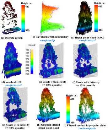
As shown in Fig. 8, we conducted a comparison of an individual tree represented by the discrete-579
return LiDAR data (Fig. 8(a)) and HPC related products. Specifically, Fig. 8(b) shows the 580
waveforms we cropped from the whole dataset using the waveformclip function. To directly 581
visualize these waveforms, the hyperpointcloud function was used to convert these waveforms into 582
the HPC as shown in Fig. 8(c). Compared to Fig. 8(a), the HPC has a larger height range with 583
more points at the top of the canopy and the bottom of the group. Furthermore, we also present the 584
HPC in a voxel format (Fig. 8(d)) coloring by intensity through the waveformvoxel function. The 585
size of the voxels is dx = 0.8, dy = 0.8 and dz = 0.15m. It can be observed that the higher intensity 586
is more likely to be located at the ground and the tree top area. While the mid-story of the tree is 587
more likely to have lower intensity. The shape of the tree crown can be vaguely recognized from 588
Fig. 8(d), however, a useful representation of individual trees with the HPC or voxels needs 589
subsequent filtering and further removal of redundant information. As an example, we presented 590
and 70% quantile (Fig. 8(g) of intensity. As anticipated, fewer voxels are left to represent the 592
vegetation structure with the increase of the intensity threshold. Interestingly, the crown shape and 593
vegetation structure can be reconstructed to some extent using filtering voxels. Especially when 594
we used 60% quantile of intensity to filter the voxels, the internal structure of the individual tree 595
can be observed. Moreover, a simple filtering strategy was implemented at the current stage. With 596
a comprehensive filtering, more representative voxels are expected. Undoubtedly, this will provide 597
an insightful way to characterize vegetation structure using waveform LiDAR data. 598
599
Fig. 8. Visualization of an individual tree using (a) discrete-return LiDAR point cloud and 600
waveform LiDAR data with different processing steps. (b) Waveforms being selected within one 601
waveforms of (b) using hyperpointcloud function; (d) Voxelization product from the HPC using 603
waveformvoxel function with res = c (0.8, 0.8 0.15) (colored by intensity); (e) Original HPC after 604
implementing intensity filtering (intensity> = 60% maximum intensity, colored by height); (f) 605
Filtered vertical HPC after using rawtocomposite function. Functions are colored in blue. 606
3.2.9 rawtocomposite 607
Most of the waveforms are not directly vertically distributed along the pulse line due to the fact 608
that the outgoing pulse was emitted at an nadir angle as shown in Fig. 8(c) and (h). This off-609
nadir angle can enhance the capability of the laser to penetrate through gaps in the forest canopy, 610
but on the other hand, it also results in the negative effect on the vegetation structure 611
characterization [13,15]. To mitigate this negative effect on the internal structure characterization, 612
we developed a new way to generate vertical waveforms from the waveform voxelization results. 613
The principle of this method is to reconstruct the raw waveforms from the products generated from 614
the waveformvoxel function. The rawtocomposite function of our package can take these voxels as 615
input and reconstruct waveforms without tilt angle (composite waveforms) based on the choice of 616
voxel intensities (maximum, mean or percentile intensity). Subsequently, composite waveforms 617
are treated as original waveforms and can recreate the HPC using the hyperpointcloud function. 618
To better demonstrate results, we present a comparison of the original HPC (Fig. 8(h) and 619
composited waveform based HPC (Fig. 8(i) after using 60% quantile intensity as the filter. We can 620
see those points in Fig. 8(i) are vertically distributed as compared to Fig. 8(h). In addition, we also 621
compared the capability of composite waveforms with the original waveforms on vegetation 622
characterization such as tree species identification (8-4). The comparisons have shown that the 623
composite waveform has an advantage over the raw waveform on the tree species identification. 624
Certainly, more efforts are needed to further test its performance and facilitate its potential 625
applications. Of particular note, the composite waveform needs additional processing steps and 626
higher computation cost, which calls for cost-benefit analysis prior to large scale application using 627
composite waveforms. Because the original waveforms may be sufficient to achieve the necessary 628
accuracy of vegetation characterization under specific circumstances. 629
The following example gave us a snapshot of how to use the rawtocomposite function to obtain 630
the composite waveforms. In addition, we provide an option to enable users to select which 631
intensity variables they want to formulate in the composite waveform. By default, we used the 632
waveforms. In the second example, we assigned inten_index to 6 which represents we used the 50% 634
percentile intensity to represent the intensity of the composite waveform. In this example (qvoxr), 635
there are eight intensity related variables were generated: the number of intensities, the maximum 636
intensity, the mean intensity, total intensity, 40th percentile intensity, 50th percentile intensity, 75th
637
percentile intensity and 86 percentile intensity in each voxel. It is important to note that the 638
resolution of composite waveform relied on the setting of the waveformvoxel function. 639
rtc<-rawtocomposite(voxr)
640
ph_rtc<-rawtocomposite(qvoxr,inten_index = 6)
641
4 Conclusion
642
The present paper aims to introduce the waveformlidar package and its applications to R users. 643
We incorporated commonly used FW processing algorithms with a new development of FW 644
LiDAR data analysis, which is expected to alleviate the technical barrier of exploring FW LiDAR 645
data and give users more flexibility to interpret results. Multiple examples are presented to 646
illustrate various features of the package. For example, several decomposition methods such as the 647
Gaussian decomposition and Gold deconvolution are available for the ecological and remote 648
sensing communities to implement sophisticated waveform processing algorithms in a comfortable 649
way. In addition, we also demonstrate a new way to directly visualize the FW LiDAR data in terms 650
of point cloud data structure and exemplify the potential usefulness of the HPC. 651
To date, only part of the functions available in waveformlidar are discussed in detail. More 652
examples of FW LiDAR data applications can be found at
653
https://github.com/tankwin08/waveformlidar. The package is still under continuous development 654
and suggestions for further features can be submitted to 655
https://github.com/tankwin08/waveformlidar/issues. 656
References
657
1. Mallet, C.; Bretar, F. Full-waveform topographic lidar: State-of-the-art. ISPRS Journal of
658
Photogrammetry and Remote Sensing 2009, 64, 1-16, doi:10.1016/j.isprsjprs.2008.09.007. 659
2. Lefsky, M.A.; Harding, D.J.; Keller, M.; Cohen, W.B.; Carabajal, C.C.; Del Bom Espirito-660
Santo, F.; Hunter, M.O.; de Oliveira, R. Estimates of forest canopy height and aboveground 661
biomass using ICESat. Geophysical Research Letters 2005, 32, 662
doi:10.1029/2005gl023971. 663
3. Allouis, T.; Durrieu, S.; Véga, C.; Couteron, P. Stem volume and above-ground biomass 664
signals. Selected Topics in Applied Earth Observations and Remote Sensing, IEEE Journal
666
of 2013, 6, 924-934. 667
4. Zhou, T.; Popescu, S.C. Bayesian decomposition of full waveform LiDAR data with 668
uncertainty analysis. Remote Sensing of Environment 2017, 200, 43-62, 669
doi:10.1016/j.rse.2017.08.012. 670
5. Hyde, P.; Dubayah, R.; Peterson, B.; Blair, J.; Hofton, M.; Hunsaker, C.; Knox, R.; Walker, 671
W. Mapping forest structure for wildlife habitat analysis using waveform lidar: Validation 672
of montane ecosystems. Remote sensing of environment 2005, 96, 427-437. 673
6. Zhou, T.; Popescu, S.C.; Krause, K.; Sheridan, R.D.; Putman, E. Gold – A novel 674
deconvolution algorithm with optimization for waveform LiDAR processing. ISPRS
675
Journal of Photogrammetry and Remote Sensing 2017, 129, 131-150, 676
doi:10.1016/j.isprsjprs.2017.04.021. 677
7. Wagner, W.; Ullrich, A.; Ducic, V.; Melzer, T.; Studnicka, N. Gaussian decomposition and 678
calibration of a novel small-footprint full-waveform digitising airborne laser scanner. 679
ISPRS Journal of Photogrammetry and Remote Sensing 2006, 60, 100-112, 680
doi:10.1016/j.isprsjprs.2005.12.001. 681
8. Wu, J.; van Aardt, J.; McGlinchy, J.; Asner, G.P. A robust signal preprocessing chain for 682
small-footprint waveform lidar. Geoscience and Remote Sensing, IEEE Transactions on
683
2012, 50, 3242-3255. 684
9. Mallet, C.; Lafarge, F.; Bretar, F.; Roux, M.; Soergel, U.; Heipke, C. A stochastic approach 685
for modelling airborne lidar waveforms. Laserscanning 2009, 201-206. 686
10. McGlinchy, J.; van Aardt, J.A.N.; Erasmus, B.; Asner, G.P.; Mathieu, R.; Wessels, K.; 687
Knapp, D.; Kennedy-Bowdoin, T.; Rhody, H.; Kerekes, J.P., et al. Extracting Structural 688
Vegetation Components From Small-Footprint Waveform Lidar for Biomass Estimation 689
in Savanna Ecosystems. IEEE Journal of Selected Topics in Applied Earth Observations
690
and Remote Sensing 2014, 7, 480-490, doi:10.1109/jstars.2013.2274761. 691
11. Isenburg, M. LAStools—Efficient tools for LiDAR processing. Available at: http:
692
http://www. cs. unc. edu/~ isenburg/lastools/[Accessed October 9, 2012] 2012. 693
12. McGaughey, R. FUSION/LDV: Software for LiDAR data analysis and visualization, 694
Version 3.01. US Department of Agriculture, Forest Service, Pacific Northwest Research
695
Station, University of Washington: Seattle, WA, USA 2012. 696
13. Zhou, T.; Popescu, S.; Lawing, A.; Eriksson, M.; Strimbu, B.; Bürkner, P. Bayesian and 697
Classical Machine Learning Methods: A Comparison for Tree Species Classification with 698
LiDAR Waveform Signatures. Remote Sensing 2017, 10, 39, doi:10.3390/rs10010039. 699
14. Zhou, T.; Popescu, S.; Malambo, L.; Zhao, K.; Krause, K. From LiDAR Waveforms to 700
Hyper Point Clouds: A Novel Data Product to Characterize Vegetation Structure. Remote
701
Sensing 2018, 10, 1949, doi:10.3390/rs10121949. 702
15. Hermosilla, T.; Ruiz, L.A.; Kazakova, A.N.; Coops, N.C.; Moskal, L.M. Estimation of 703
forest structure and canopy fuel parameters from small-footprint full-waveform LiDAR 704
data. International journal of wildland fire 2014, 23, 224-233. 705