Article
1
High Reliable and Efficient Three Layer Cloud
2
Dispatching Architecture in the Heterogeneous
3
Cloud Computing Environment
4
5
Mao-Lun Chiang 1, Yung-Fa Huang 1,*, Hui-Ching Hsieh2 and Wen-Chung Tsai1
6
1 Department of Information and Communication Engineering, Chaoyang University of Technology,
7
Taichung City, Taiwan ROC; {mlchiang, yfahuang, azongtsai}@cyut.edu.tw
8
2 Department of Information and Communication, Hsing Wu University of Technology, New Taipei City,
9
Taiwan, ROC; [email protected]
10
* Correspondence: [email protected]; Tel.: +886-423323000-7243
11
12
Featured Application: Authors are encouraged to provide a concise description of the specific
13
application or a potential application of the work. This section is not mandatory.
14
Abstract: Due to the rapid development and popularity of the Internet, cloud computing has
15
become an indispensable application service. However, how to assign various tasks to the
16
appropriate service nodes is an important issue. Based on the reason above, an efficient scheduling
17
algorithm is necessary to enhance the performance of system. Therefore, a Three-Layer Cloud
18
Dispatching (TLCD) architecture is proposed to enhance the performance of task scheduling. In first
19
layer, the tasks need to be distinguished to different types by their characters. Subsequently, the
20
Cluster Selection Algorithm is proposed to dispatch the task to appropriately service cluster in the
21
secondly layer. Besides, a new scheduling algorithm is proposed to dispatch the task to a suitable
22
server in a server cluster to improve the dispatching efficiency in the thirdly layer. Basically, the
23
TLCD architecture can obtain better task completion time than previous works. Besides, our
24
algorithm and can achieve load-balancing and reliability in cloud computing network.
25
26
Keywords: cloud computing, reliability, load balancing, Sufferage, task dispatching
27
28
1. Introduction
29
Due to the rapid development and popularity of the Internet, cloud computing has become an
30
indispensable and highly-demanded application service [1]. In order to meet the more storage
31
requirement of big data, the system will continue to upgrade and expand its capabilities, resulting in
32
a large number of heterogeneous servers, storage and related equipment in a cloud computing
33
environment.
34
Furthermore, the cloud computing network can be divided into three basic service categories:
35
The Software as a Service (SaaS), the Platforms as a Service (PaaS) and the Infrastructure as a Service
36
(IaaS) [2][3[4]. In SaaS, the software is provided by the software vendor, such as Gmail and Google
37
Driver. For the PaaS, it provides a platform for users for programming purpose. Google APP Engine
38
is one kind of platforms of PaaS. In the last category of service called the IaaS, the hardware resources
39
are proposed to support users for constructing the framework, such as Cloud server [2][3[4] No
40
matter what kind of cloud service is applied to the cloud computing network, there has a common
41
character: each server has different ability and computing power. Therefore, propose an efficient
42
scheduling algorithm for dispatching the tasks to appropriate server nodes of cloud becomes an
43
important challenge in cloud computing network.
44
Basically, in the traditional cloud clustering architecture, system only considers the
45
heterogeneity of tasks while executing scheduling procedure and ignores the heterogeneity of tasks
46
which come from different platforms and its categories are not distinguishable by nodes. Therefore,
47
heterogeneous tasks have become major flaws in traditional cloud architectures. In addition, cloud
48
service types are very diverse. As a result, the cloud computing environment becomes complicated
49
and the reliability is greatly reduced. So, the scheduling of cloud environments is more difficult.
50
Therefore, the Three-Layer Cloud Dispatching (TLCD) architecture is proposed to handle the
51
scheduling problem while the heterogeneous nodes and tasks exist in the cloud system at the same
52
time. For the first layer, Category Assignment Cluster (CAC) [6][7] layer was proposed to reduce the
53
task delay and the overloading by classifying the heterogeneous tasks. In CAC layer, the various
54
tasks can be classified as three types according to the IaaS, SaaS, and PaaS categories. Subsequently,
55
the homogeneous tasks can be dispatched to corresponding service category clusters in the second
56
layer.
57
In the second layer, called the Cluster Selection (CS) layer, the homogenous task can be assigned
58
to appropriate cluster by Cluster Scheduling Algorithm (CSA) to enhance the reliability of system.
59
Besides, the cost and completion time of task scheduling can be reduced in this layer.
60
Finally, tasks can be dispatched to service nodes by scheduling algorithm in the third layer,
61
Server Nodes Selection (SNS) layer. In this layer, an Advanced Cluster Sufferage Scheduling (ACSS)
62
algorithm is proposed to enhance the resource utilization and to achieve load balancing
63
[2][3][8][9][10][11].
64
The rest of this paper is organized as follows. Section 2 will describe the related works of
65
scheduling algorithms in the cloud computing network. Section 3 gives the explanation of the TLCD
66
architecture and the proposed algorithm. In section 4, an example is provided to describe the overall
67
procedure of ACSS. Finally, the conclusions is given in Section 5.
68
69
2. Materials and Methods
70
In general, scheduling algorithm is a mapping mechanism and is being divided into two modes:
71
the real-time mode and the batch mode. The main difference between these two modes is the timing
72
of dispatching. Basically, tasks in the real-time mode will be assigned to server nodes immediately.
73
In contrast to real-time mode, tasks will be assigned to server once the number of tasks is accumulated
74
to a certain amount under the batch mode. In other words, the real-time scheduling algorithm only
75
focuses on the results of a single task assignment, while the batch scheduling algorithm considers the
76
assignments results of all tasks. Therefore, the batch mode scheduling algorithm has better
77
performance in load balancing and completion time than the real-time scheduling algorithm
78
[11][12][13].
79
So far, many mechanisms have been proposed to ensure the quality of service in the cloud
80
computing network, and an appropriate task scheduling algorithm is one of the most important
81
methods to achieve these goals. During the last several decades, there has been an increase in the
82
number of publications on task dispatching algorithms [2][3][8][9][10][12][14]. Basically, these
83
algorithms, such as Min-Min [8][9][12][14], Max-Min[8][12][14]14, Sufferage [2][8][10][14] and
84
MaxSufferage algorithm[2][3][8][12], only consider the expected completion time (ECT) as a factor
85
while designing the scheduling algorithm. The load status of the node is not considered. Therefore,
86
the completion time is not as expected.
87
For example, in Min-Min algorithm, the tasks of the smallest sets are selected. With the selected
88
set, the task which has the smallest ECT value will be assigned to the server nodes. It starts with a set
89
T of all unassigned tasks and the task with minimum completion time is selected as min_ECTi. Then,
90
the task with overall minimum completion time from min_ECTi is selected and assigned to that server
91
node. Finally, the newly mapped task is removed from T and the process repeats until all tasks are
92
assigned. Under such algorithm, the network system will be unbalanced while there have too many
93
Similar to Min-Min algorithm, the completion time is also an estimated factor for dispatching
95
tasks under Max-Min algorithm. The difference between these two algorithms is that Max-Min
96
algorithm selects the tasks with overall maximum completion time instead of the minimum
97
completion time. However, the large tasks are always to be assigned in advance in Max-Min
98
scheduling algorithm. Hence, the overall completion time will increase significantly [8][12][14].
99
Basically, the server nodes with higher ability are easily to be assigned more tasks than the server
100
nodes with lower ability in the above algorithms. Therefore, the workloads of server nodes are
101
unbalanced and the completion time will increase significantly. As a result, the Sufferage algorithm
102
[1][14][15][16] is proposed to improve the load balancing of the network system. Here, the main
103
concept of Sufferage algorithm is dispatching the tasks to server nodes by computing the Sufferage
104
Value(SV)which is calculated by the second earliest completion time minus the earliest completion
105
time. Subsequently, task i with largest SV value will be assigned to the appropriate server nodes with
106
minimum ECT. However, the completion time between tasks cannot be reduced effectively and the
107
load balancing cannot be improved while there are too many tasks waiting for dispatching.
108
Based on the reason above, the MaxSufferage algorithm 3 is proposed to improve the defect of
109
Sufferage algorithm, and the proposed protocol is divided into three phases. In the first phase called
110
the SVi calculation phase, the SV value is calculated among all of tasks. Following is the MSVi
111
calculation phase, and the task i with the second earliest ECT will be elected as MaxSufferage
112
Value(MSV) value while task i has the maximum SV value among all SV values. For the last phase
113
called the task dispatch phase, task i with minimum ECT can be dispatched to appropriate server
114
node j when MSVi > ECTij of server node j. Conversely, task i with a maximum ECT value can be
115
dispatched to server node j. Unfortunately, the large tasks are easy to be dispatched to server nodes
116
with poor ability in MaxSufferage algorithm under the heterogeneous environments
117
For solving the problem above, the AMS algorithm[17] to improve the drawback of
118
MaxSufferage algorithm. However, the AMS only considers the task scheduling of service nodes,
119
regardless of the cluster and type of service. As a result, an incremental algorithm is proposed to
120
solve the scheduling service types, clusters, and service nodes simultaneously. Besides, all the tasks
121
be dispatched to the appropriate server nodes in the cloud computing network even if the server
122
nodes are located in heterogeneous environment.
123
Subsequently, the related description of our algorithm and explained as follow.
124
125
3. Three-layer cloud dispatching Architecture
126
127
Since the traditional dispatch algorithm of cluster architecture does not dispatch task by its
128
capacity of cluster. It may cause the drawback of task delay, low reliability and high MakeSpan.
129
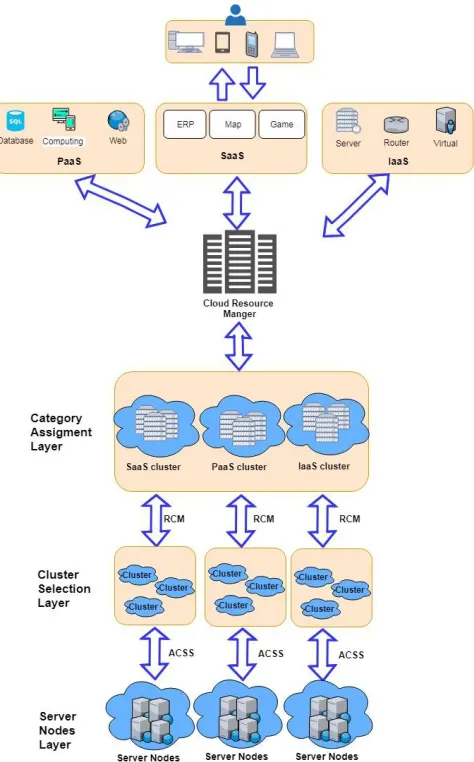
Therefore, a Three Layer Cloud Dispatching (TLCD) architecture and related scheduling algorithm
130
are proposed to apply to cluster-based cloud environment, as shown in Figure. 1. The description of
131
Figure. 1 .Three Layer Cloud Dispatching Architecture
133
134
3.1 Category Assignment cluster layer
135
The traditional cluster architecture collects and distributes tasks to the cluster by cloud resource
136
managers. But, the allocation process may be affected by cluster heterogeneity, causing the task to be
137
insignificant in terms of scheduling. It is because that the tasks are allocated to idle cluster by cloud
138
resource managers. Therefore, the scheduling result is not ideal. This will increase the complexity of
139
the cloud computing system.
140
Besides, the diversity of tasks increases the delay of processing time. To reduce the delay and
141
the complexity of scheduling, the heterogeneity task can be classified into different categories
142
according to demand defined in Category Assignment Cluster (CAC) layer [6][7]. The category cloud
143
clusters can be divided into three types: SaaS, PaaS and IaaS. Through these three categories of
144
classification, the difficulty of scheduling on heterogeneous tasks and scheduling delays can be
145
reduced.
146
147
3.2 Cluster selection layer
148
149
After completing the classification of the category assignment cluster layer, the classified tasks
150
can be dispatched to the corresponding category cluster. Subsequently, a Cluster Selection Algorithm
151
(CSA) is proposed to assign the tasks to appropriate cluster by using the factors of Reliability (Ri),
152
Cost (Ci) and MakeSpan (Mi) [3][18]. MakeSpan is the length of time to complete a task. Basically,
when the MakeSpan value is getting bigger, the system will need longer operation time. Due to the
154
similarity of the fault-tolerance of clusters, the computing power will increase as the Reliability gets
155
higher. Therefore, we need to focus on clusters' computing power [3][18]. Finally, for the cost factor,
156
it is defined as the cost needed for a task to be sent and responded. When taking these three factors
157
into account, tasks can be assigned to suitable cluster and the system efficiency can be enhanced. In
158
addition, users and service providers can customize those three factors based on their own
159
requirements. According to the above description, in the following example, we customize the
160
Reliability (Ri) and Cost (Ci), and arrange the tasks to the suitable clusters. Because, the objectives of
161
this example are configured for reliability and cost. Subsequently, we propose an example to explain
162
this algorithm.
163
164
Ri = (∑ _ ) / n (1)
165
= (∑ _ ) (2)
166
= (∑ _ )/n (3)
167
168
k = cluster k.
169
i = assignment i.
170
n = the total number of tasks
171
l = the total number of clusters
172
= the number of tasks assigned to the k cluster.
173
_ = the reliability of the cluster k.
174
_ = the makespan of the cluster k.
175
Sub_Ck= the cost of the cluster k.
176
177
In Line (4), we arranged the combination of tasks in all clusters. Cluster will choose an
178
appropriate task combination and then help node to adjust these tasks. Furthermore, line (5) to (8)
179
are proposed to check if the and of each assignment i agree with Ri ≥ Rs && Ci ≥ Cs. Then among
180
those passed assignments, the one with the smallest is scheduled. If there are more than two
181
groups eligible, we compare Ri and Mi and choose Ai as the combination of the highest reliability and
182
the least time.
183
In CSA, users can customize the quality of services by reliability, cost and MakeSpan factors.
184
Thus, algorithms can meet the requirements of various users and can enhance the efficiency of job
185
scheduling.
186
Subsequently, an example is shown to explain CSA algorithm and the related assumptions are
187
showing in Table 1.
188
189
Algorithm 1-
Cluster Selection Algorithm
= .
=
=
=
=
=
=
=
: for
2: for total cluster k
4: Arrange all tasks in the cluster and assign the number of Ai
5: for calculating the 、 and Mi of the assignment
6: if ≥ && < in assignment then is candidate assignment
7: end for
8: choose the smallest in candidate assignment
9: end for
:
:
190
191
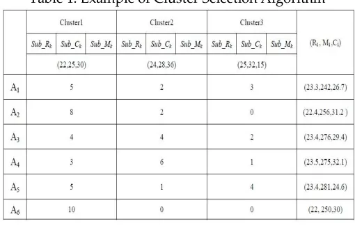
Table 1. Example of Cluster Selection Algorithm
192
193
194
We assumed that there are 10 tasks need to be sent to 3 cloud clusters, the process is the
195
following:
196
197
Step 1: Rs and Cs are set by user. In this example, Rs and Cs. are 22 and 260 respectively.
198
199
Step 2: Calculate Ri, Ci and Mi of each allocation combination. According to Table 1, assignment
200
A1 assign five tasks to Cluster 1, two tasks to Cluster 2 and three tasks to Cluster 3 respectively We
201
used formula (1) and (2) to calculate the average of Ri, Ci and Mi, and showing as follows.
202
203
=22 × 5 + 24 × 2 + 25 × 3
10 = 23.3
204
205
C1 = 25 × 5 + 28 × 2 + 32 × 3 = 242
206
207
M =30 × 5 + 36 × 2 + 15 × 3
10 = 26.7
208
209
The same procedure goes to other assignments too.
210
211
Step 3: Select the schedule that meets the condition of Ri ≥ 22 and Ci < 260; Here, A1、A2 and A6
212
are selected.
213
214
Step 4: According to the conditions of step 3, we choose A1 with the highest reliability and
215
smallest MakeSpan. Since the result of assignment A1 is better than others, thus assignment A1 is
216
The above procedure is the most suitable solution when the MakeSpan is the main concern.
218
However, when the reliability is the main concern, the MakeSpan and Cost become the masking
219
factors to filter out the schedule with the best reliability. After finished the CSA layer, the tasks can
220
be dispatched to the corresponding clusters in cloud cluster section layer. Subsequently, the
221
appropriate server nodes need to be elected to complete the task in the next layer.
222
223
3.3 Server nodes selection layer
224
225
After finishing the first two layers, the homogeneous tasks can be dispatched to homogeneous
226
cloud cluster. However, tasks may be assigned to inappropriate server nodes when there exists a
227
large number of tasks. As a result, system will become unbalanced and will have higher completion
228
time. To solve these problems, the Advanced Cluster Sufferage Scheduling (ACSS) algorithm is
229
proposed to improve the defect of MaxSufferage algorithm [12][14][15] under the heterogeneous
230
cloud computing network. The main concept of ACSS algorithm is making the tasks dispatched to
231
the appropriate server nodes by using the average ECT of server node denoted as Sj to reduce the
232
influence of inappropriate assignment. The detail of ACSS algorithm is shown in Algorithm 2.
233
Basically, the ACSS algorithm is divided into three phases. In the first phase called the SVj
234
calculation phase, system will find the (The earliest expected completion time) and
235
(The second earliest expect completion time) of the Sj to calculate the SV value, and the detail
236
procedure is shown in lines (8) ~ (9) in Figure 3. Subsequently, the MSV value will be set to the second
237
earliest ECT value of task i in the second phase which is called as the MSVi calculation phase while
238
task i has the maximum SV value among all SV values.
239
In the third phase called the task dispatching phase, task i will be dispatched to Sj while MSVi >
240
ECTij and EECTiECT >AECTj of Sj. Conversely, when EECTiECT ECTi1st< AECTj, task i can be
241
dispatched to server node j where the ECT is approximate to AECTj and the ECTneeds to be larger
242
than AECTj. Basically, the procedure is different from Sufferage and MaxSufferage algorithm, and
243
the detail algorithm is shown in line (11) and (12) in Algorithm 2.
244
245
Algorithm 2 Advanced Cluster Sufferage Scheduling
=the task completion time of the task i in the server node ;
=the expected completion time of task i in the server node ;
= the expected time of server node will become ready to execute for next task;
= the expected completion time of Average time in the server node ;
= the earliest expected completion time of tasks i;
= the second earliest expected completion time of task i;
= ;
= ;
1:
2:
3: = +
4:
5: mark all server nodes as unassigned;
6: for each task i in ;
7: find server node that gives the earliest completion time;
8: calculating the Sufferage Value ( = − );
then chose the assignment to MSV with maximum;
elsethe assignment i with maximum can be compared to other ;
10: If( < )
Then the task i with maximum ECT can be dispatched to server nodes ;
11: else if( > ) && ( > )
then the task i can be dispatched to server nodes ;
12: else if(MSVi >ECTij) && ( < )
Then assignment task i > _ && ≈ can be dispatched to server nodes Sj ;
13: end if;
14: end for
15: = +
16: = +
17: end do
246
According to the operations above, the completion time and load balancing of the heterogeneous
247
cloud computing network can be improved efficiently. For the security issue, we can hire a MAC
248
algorithm [15][19] with session key to confirm that the message come from the truly sender and has
249
not been modified. Subsequently, the example is provided to help understanding the ACSS algorithm
250
of server node selection layer.
251
252
4. Example and comparison results
253
In this paper, four heterogeneous environments including HiHi (High heterogeneity task, High
254
heterogeneity server node), HiLo, LoHi and LoLo [4, 10] will be discussed. Basically, HiHi is the most
255
complex problem. Hence, in this paper, we will use four nodes and twelve tasks for task assignment
256
under the HiHi's heterogeneous environment as an example. Subsequently, the ACSS algorithm
257
assignment task process can be divided into three phases to show our processes. Firstly, the SV value
258
and the MSV value can be calculated in the SVj calculation phase and the MSVi calculation phase. The
259
dispatching procedure is executed in the task dispatching phase by using AECTj of SN . The
260
parameters of HiHi environment are shown in Table 2.
261
262
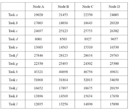
Table 2. Illustrations of the expected execution time of tasks
263
264
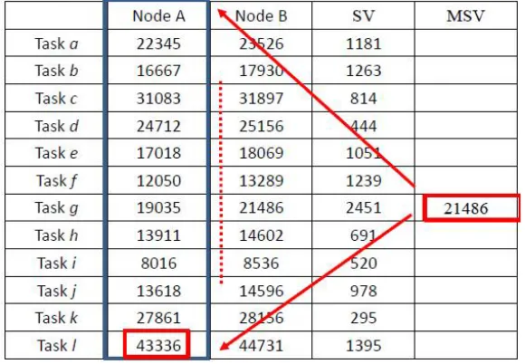
The SVi calculation phase
279
Step 1. List the expected execution times for all task i on Sj, as shown in Table 2.
280
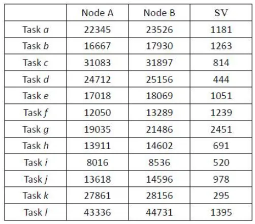
Step 2. Calculate the SV value for each task. For example, the SV value of Task a is equal to
281
SEECTi minus EECTi, which is 23526-22345 = 1181, and the same procedures will be executed for
282
task b to l to calculate the SV values. The calculation results are shown in Table 3.
283
284
Table 3. Calculation of the SV value of tasks
285
286
287
288
The MSVi calculation phase
289
Step 1. The second earliest ECT value of Task i can be selected as MSV value while task i has the
290
maximum SVi value among all SV values. As shown in Table 4, the task with the largest SVi value is
291
Task g, thus the second earliest ECT (Here is 21486) of ECTgB is selected as the MSV value.
292
293
Table 4. Calculation of the MSV value of tasks
294
295
296
297
Basically, there are three cases that need to be discussed in different heterogeneous
299
environments, and the cases are illustrated and discussed as follows step by step.
300
301
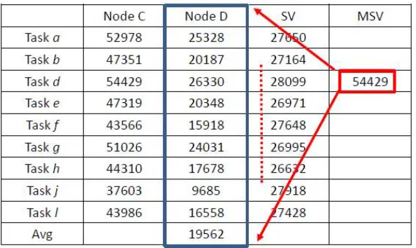
Case 1 MSVi > ECTij of Sj and EECTi > AECTj of Sj
302
Compare the MSV value founded in the MSVi calculation phase with the earliest expected
303
completion time of other tasks. Task i can be dispatched to the appropriate server node j while MSVi
304
> ECTij of Sj and EECTi > AECTj of Sj. Therefore, task d is dispatched to Node D while the MSVi > ECTdD
305
and ECTdD > AECTj in table 5 and table 6.
306
307
Table 5. Comparison of the MSV value of tasks
308
309
310
311
Table 6. Comparison of the average ECT of tasks in Node D under case 1
312
313
314
315
316
Case 2. MSVi < ECTij of Si
317
318
Compare the MSV value founded in the MSVi calculation phase with the earliest expected
319
completion time of other tasks. Task i with maximum ECT can be dispatched to appropriate server
320
node j when MSVi < ECTij of server node j. Therefore, task l is assigned to Node A in Table 7 because
321
its ECTlA is greater than the MSV value (43336> 21486).
322
323
324
326
327
Case 3. MSVi > ECTij of Sj and EECTi < AECTj of Sj
328
329
Compare the MSV value founded in the MSVi calculation phase with the earliest expected
330
completion time of other tasks. Task i in table 8 will be dispatched to server node j where the ECTi
331
is approximate to AECTj and the ECTi is larger than AECTj under the conditions that the MSVi >
332
ECTij and EECTi < AECTj of Sj. Therefore, task j is assigned to Node B in table 9 because ECTjB is bigger
333
than and closer to AECTB.
334
335
Table 5. Comparison of the average ECT of tasks in Node D under case 3
336
337
338
339
Table 9. Assign tasks to the server nodes
340
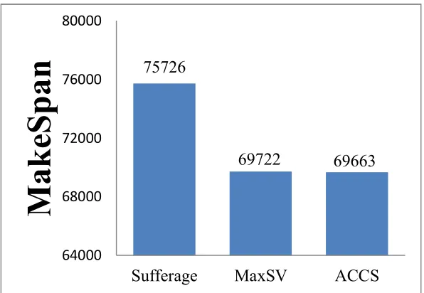
Based on the examples above, the comparisons of MakeSpan and load balancing among the
343
Sufferage, MaxSufferage, and ACSS algorithms are shown in Figure 2 to 5. In Figure. 2, the proposed
344
algorithm has better MakeSpan than others. In addition, the load balancing index can be calculated
345
by using the following formula [1][12].
346
Load balance index =rmin/rmax
347
=The shortest completed task time of all tasks.
348
=The longest completed task time of all tasks.
349
350
Basically, the value of load balancing index will be a number between 0 and 1. Here, 0 represents
351
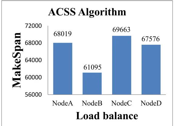
the worst load balancing and 1 represents the best.
352
As shown in the Figure. 3 to 5, ACSS algorithm can obtain best load balancing index (0.88) which
353
is better than Sufferage (0.87) and MaxSufferage (0.83). Because the ACSS algorithm uses the
354
distribution of the average value, the Makespan of each node can achieve similar results. However,
355
MaxSufferage completed time is better than Sufferage, but the load balancing results are similar. This
356
is because that MaxSufferage did not consider the load status of the node during the selection of tasks.
357
Thus, the proposed ACSS algorithm is more adapted to the heterogeneous cloud computing network
358
than other algorithms.
359
360
Besides, the formula =∑ × 100%is used to calculate ratio of resource utilization to
361
show whether the use of resource in this paper is maximized. In factor RU, the represents the
362
total expected completion time by virtual machine j; N represents the number of virtual machines
363
and m represents the final completion time of the virtual machine. And, the related ratio results of
364
resource utilization are shown in Figure. 6. In Figure. 6, the ratio of resource utilization of ACCS can
365
reach 89%, and this result is better than others. It is because that the average value is used to consider
366
allocation status of nodes in ACSS algorithm
367
Subsequently, the parameter of matching proximity is used to evaluate the degree of proximity
368
of vary schedule algorithms. In Figure. 7, the MET (Minimum Execution Time) and ECT (Expected
369
Compute Time) are used to estimate whether the task can be to quickly matched. A large value for
370
matching proximity means that a large number of tasks are assigned to the machine that executes
371
them faster [10]. The formula (4) is shown as follow.
372
373
Matching Proximity = ∑∑∈ [ ][ ] [ ][ ]
∈ (4)
374
375
As show in Figure. 7, the matching ratio of the three algorithms is close to 1. These three
376
algorithms have good matching efficiency.
377
Subsequently, the performance of algorithms can be compared in Table 10. The results of
378
comparison table show that ACSS can obtain the best performance among all algorithms in
379
evaluation factors including Makespan, load balance, resource utilization and matching proximity.
380
384
385
Figure. 2. The comparison results of MakeSpan
386
387
388
389
390
Figure. 3. The load balancing index in Sufferage scheduling algorithm
391
392
393
Figure. 4. The load balancing index in MaxSufferage scheduling algorithm
394
395
75726
69722
69663
64000 68000 72000 76000 80000
Sufferage
MaxSV
ACCS
M
ak
eS
p
an
75786
68257
66353
65806
60000 64000 68000 72000 76000 80000
NodeA
NodeB
NodeC
NodeD
M
a
k
eS
p
a
n
396
Figure. 5. The load balancing index in ACSS scheduling algorithm
397
398
399
400
Figure. 6. The ratio of Resource Utilization in ACSS scheduling algorithm
401
402
403
404
Figure. 7. The ratio of Matching Proximity in all of scheduling algorithms
405
406
Table 10. The performance comparison of all of algorithms
407
408
68019
61095
69663
67576
56000 60000 64000 68000 72000
NodeA
NodeB
NodeC
NodeD
M
a
k
eS
p
a
n
Sufferage
MaxSufferage
ACSS
Experiments
MakeSpan
75726
69722
69663
Load
Balance
0.87
0.84
0.88
Resource
Utilization
91%
95.5%
96%
Matching
Proximity
0.97
0.965
0.963
409
5. Conclusions
410
Recently, cloud service users gradually increased, how to provide an efficient service for users
411
is still an important issue. In this study, the TLCD architecture is proposed to provide secure and
412
reliable scheduling and to improve the defect of the slow response of the cloud system.
413
Basically, TLCD includes three layers of procedure. In the first layer which is called the CAC
414
layer, system can dispatch the heterogeneous tasks into appropriate category clusters to reduce task
415
delay and overloading. Subsequently, a CSA algorithm is proposed in CS layer to dispatch the task
416
to appropriate Cluster to enhance the reliability and reduce the cost and completion time. In the final
417
layer which is defined as the SNS layer, system can improve the load balancing and reduce the
418
completion time by elements of MSV and the average ECT of Sj.
419
Finally, as shown in Table 10, the proposed algorithms can obtain best results among all
420
algorithms in evaluation factors including makespan, load balance, resource utilization and matching
421
proximity under the heterogeneous environments.
422
Author Contributions: A and B designed the framework and wrote the manuscript. C and D verified the results
423
of our work and conceived the experiments together. All authors discussed the results and contributed to the
424
final manuscript.
425
References
426
1. Petkovic, I. CRM in the cloud. In Proceedings of the IEEE 8th International Symposium on Intelligent
427
Systems and Informatics, September 2010; pp. 365-370.
428
2. Casanova, H.; Legrand, A.; Zagorodnov, D.; Berman, F. Heuristics for scheduling parameter sweep
429
applications in grid environment. In Proceedings of the 9th Heterogeneous Computing Workshop, Cancun,
430
Mexico, May 2000; pp. 349-363.
431
3. Chiang, M.L.; Luo, J.A.; Lin, C.B. High-Reliable Dispatching Mechanisms for Tasks in Cloud Computing.
432
In Proceedings of the BAI2013 International Conference on Business and Information, Bali, Indonesia, 7-9
433
July 2013; pp. 73.
434
4. Buyya, R.; Ranjan, R.; Calheiros, R.N. Modeling and simulation of scalable Cloud computing environments
435
and the CloudSim toolkit: Challenges and opportunities. In Proceedings of the International Conference
436
on High Performance Computing & Simulation, Leipzig, Germany, June 2009; pp. 1-11.
437
5. Lee, Y. H.; Huang, K. C.; Wu, C. H.; Kuo, Y. H.; Lai, K. C. A Framework of Proactive Resource Provisioning
438
in IaaS Clouds. Appl. Sci. 2017, 7(8), 777.
439
6. Alfazi, A.; Sheng, Q.Z.; Qin, Y.; Noor, T.H. Ontology-Based Automatic Cloud ServiceCategorization for
440
Enhancing Cloud ServiceDiscovery. In Proceedings of the IEEE 19th International Enterprise Distributed
441
Object Computing Conference, Sept 2015; 151-158.
442
7. Salton, G.; Buckley, C. Term-weighting approaches in automatic text retrieval. Inf. Process. Manage. Aug
443
8. Reda, N.M.; Tawfik, A.; Marzok, M.A.; Khamis, S.M. Sort-Mid tasks scheduling algorithm in grid
445
computing. Journal of Advanced Research. November 2015, 6, 6, 987-993.
446
9. Anousha, S.; Ahmadi, M. An improved Min-Min task scheduling algorithm in grid computing. Lecture
447
Notes in Computer Science Grid and Pervasive Computing. May 2013, 7861, 103-113.
448
10. Merajiand, S.; Salehnamadi, M.R. A batch mode scheduling algorithm for grid computing. Journal of Basic
449
and Applied Scientific Research 2013, 3, 4, 173-181.
450
11. Meraji, S.; Reza Salehnamadi, M. A Batch Mode Scheduling Algorithm for Grid Computing. Journal of
451
Basic and Applied ScientificResearch 2013,3, 4, 174-176.
452
12. Maheswaran, M.; Ali, S.; Siegel, H.J.; Hensgen, D.; Freund, R.F. Dynamic Mapping of a Class of
453
Independent Tasks onto Heterogeneous Computing Systems. Journal of Parallel and Distributed
454
Computing November 1999, 59, 2, 107-131.
455
13. Braun, T.D.; et al. A comparison study of static mapping heuristics for a class of meta-tasks on
456
heterogeneous computing systems. In Proceedings of the Heterogeneous Computing Workshop (HCW '99)
457
DC, USA, May 1999; pp. 15-29.
458
14. Etminani, K.; Naghibzadeh, M. A Min-Min Max-Min selective algorithm for grid task scheduling. In
459
Proceeding of the Third IEEE/IFIP International Conference in Central Asia on Internet, September 2007;
460
pp. 138-144.
461
15. Lan, J.; Zhou, J.; Liu, X. An area-efficient implementation of a Message Authentication Code (MAC)
462
algorithm for cryptographic systems. In Proceeding of the IEEE Region 10 Conference (TENCON), Nov
463
2016; pp. 1977-1979.
464
16. Li S.; Liu, J.; Wang, S.; Li, D.; Huang, T.; Dou, W. A Novel Node Selection Method for Real-Time
465
Collaborative Computation in Cloud. In Proceedings of the International Conference on Advanced Cloud
466
and Big Data (CBD), Aug 2016; pp. 98-103.
467
17. Chiang, M. L.; Hsieh, H. C.; Tsai, W. C.; Ke, M. C. An Improved Task Scheduling and Load Balancing
468
Algorithm under the Heterogeneous Cloud Computing Network. In Proceeding of the IEEE 8th
469
International Conference on Awareness Science and Technology (iCAST2017), Taichung Taiwan, 8-10 Nov.
470
2017; pp. 61.
471
18. Deng, J.; Huang, S.C.H.; Han, Y.S.; Deng, J.H. Fault-Tolerant and Reliable Computation in Cloud
472
Computing. In Proceedings of the IEEE Globecom 2010 Workshop on Web and Pervasive Security, Dec
473
2010; pp. 1601-1605.
474
19. Yoon, E.J.; Yoo, K.Y. An Efficient Diffie-Hellman-MAC Key Exchange Scheme. In Proceedings of the Fourth
475
International Conference on Innovative Computing, Information and Control (ICICIC), Dec. 2009; pp.
398-476
400.
477