Rothamsted Research is a Company Limited by Guarantee Registered Office: as above. Registered in England No. 2393175. Registered Charity No. 802038. VAT No. 197 4201 51. Founded in 1843 by John Bennet Lawes.
Rothamsted Repository Download
A - Papers appearing in refereed journals
Todman, L. C., Coleman, K., Milne, A. E., Gil, J. D. B., Reidsma, P.,
Schwoob, M-H., Treyer, S. and Whitmore, A. P. 2019. Multi-objective
optimization as a tool to identify possibilities for future agricultural
landscapes. Science of the Total Environment. 687 (15 October), pp.
535-545.
The publisher's version can be accessed at:
•
https://dx.doi.org/10.1016/j.scitotenv.2019.06.070
The output can be accessed at: https://repository.rothamsted.ac.uk/item/8ww1x.
© 6 June 2019, the authors. Licensed under the Creative Commons CC BY.
Multi-objective optimization as a tool to identify possibilities for
future agricultural landscapes
Lindsay C. Todman, Kevin Coleman, Alice E. Milne, Juliana D.B.
Gil, Pytrik Reidsma, Marie-Hélène Schwoob, Sébastien Treyer,
Andrew P. Whitmore
PII:
S0048-9697(19)32638-5
DOI:
https://doi.org/10.1016/j.scitotenv.2019.06.070
Reference:
STOTEN 32724
To appear in:
Science of the Total Environment
Received date:
20 February 2019
Revised date:
22 May 2019
Accepted date:
4 June 2019
Please cite this article as: L.C. Todman, K. Coleman, A.E. Milne, et al., Multi-objective
optimization as a tool to identify possibilities for future agricultural landscapes, Science of
the Total Environment,
https://doi.org/10.1016/j.scitotenv.2019.06.070
ACCEPTED MANUSCRIPT
1
Multi-objective optimization as a tool to identify possibilities for future
agricultural landscapes.
Authors: Lindsay C. Todman1*, Kevin Coleman1, Alice E. Milne1, Juliana D. B. Gil2, Pytrik Reidsma2,
Marie-Hélène Schwoob3, Sébastien Treyer3, Andrew P. Whitmore1
1
Rothamsted Research, Harpenden, Hertfordshire AL5 2JQ, UK
2
Plant Production Systems group, Wageningen University, The Netherlands
3 Institut du Développement Durable et des Relations Internationales (IDDRI), 41 Rue du Four,
75006 Paris, France
*Corresponding Author Email: [email protected]. Present address: School of Agriculture,
Policy and Development, University of Reading, PO Box 237, Earley Gate, Reading, Berkshire, RG6
6AR
Abstract
Agricultural landscapes provide many functions simultaneously including food production, regulation
of water and regulation of greenhouse gases. Thus, it is challenging to make land management
decisions, particularly transformative changes, that improve on one function without unintended
consequences on other functions. To make informed decisions the trade -offs between different
landscape functions must be considered. Here, we use a multi-objective optimization algorithm with
a model of crop production that also simulates environmental effects such as nitrous oxide
emissions to identify trade-off frontiers and associated possibilities for agricultural management.
Trade-offs are identified in three soil types, using wheat production in the UK as an example, then
the trade-off for combined management of the three soils is considered. The optimisation algorithm
identifies trade-offs between different objectives and allows them to be visualised. For example, we
ACCEPTED MANUSCRIPT
2
where small changes might have a large impact. We used a cluster analysis to identify distinct
management strategies with similar management actions and use these clusters to link the trade -off
curves to possibilities for management. There were more possible strategies for achieving desirable
environmental outcomes and remaining profitable when the management of different soil types was
considered together. Interestingly, it was on the soil capable of the highest potential profit that
lower profit strategies were identified as useful for combined management. Meanwhile, to maintain
average profitability across the soils, it was necessary to maximise the profit from the soil with the
lowest potential profit. These results are somewhat counterintuitive and so the range of strategies
supplied by the model could be used to stimulate discussion amongst stakeholders. In particular, as
some key objectives can be met in different ways, stakeholders could discuss the impact of these
management strategies on other objectives not quantified by the model.
Highlights
Trade-offs between different objectives in agricultural landscapes are complex
Cluster analysis helped visualise effects of management on trade-offs
Minimum N2O emissions scaled linearly with yield until ~85-90% of maximum yield
A more fertile soil could be managed more flexibly and remain profitable
Achieving profitability on the least fertile soil was key for overall profitability
ACCEPTED MANUSCRIPT
3
Introduction
The United Nations Sustainable Development Goals (SDGs) set out an ambitious suite of targets t o
stimulate effort to improve sustainability globally. Core to the SDGs is that these targets should not
be considered in isolation, but that the interlinkages between the goals should be accounted for. The
agricultural sector plays an important role in achieving many of the goals, most obviously ‘zero
hunger' which cannot be achieved without food production, but also impacts on goals relating to the
environment (Gil et al., 2018) such as ‘life on land’, ‘climate action’ and ‘end poverty’. Indeed,
agricultural production systems have been identified as a major contributor to key global issues such
as biodiversity loss, climate change and unsustainable nutrient cycling (Steffen et al, 2015; Burns et
al., 2016; Campbell et al., 2017). This has led to increasing interest in understanding how agricultural
production systems could be transformed to reduce negative environmental impacts whilst
providing nutritious food and prosperous livelihoods within the sector (Kanter et al., 2018). Yet the
complexity of these systems, their global scale and even their variability at local scale is a barrier to
transformative change because it is difficult to identify alternatives to the current situation that take
account of all the processes that might be affected by change and the multiple functions of
agricultural landscapes.
One particular challenge is to stimulate informed stakeholder discussion about trade -offs within
agricultural landscapes so that priorities can be identified collectively. This requires information
ACCEPTED MANUSCRIPT
4
systems to meet different combinations of objectives. Various methods have been used for
identifying trade-offs in agricultural systems, including participatory methods, empirical methods,
the use of multi-objective algorithms with models of agricultural systems and combinations of the
above (Klapwijk et al., 2014). Multi-objective algorithms are appealing because they can make use of
the current understanding of systems that is embedded in models. They may need to be combined
with other methods where key processes and objectives are not adequately represented in models.
Optimization algorithms strategically try different configurations of land management (the inputs to
a model of an agricultural system) to identify an optimal value of a quantifiable objective or
objectives (the outputs from the model). Multi-objective algorithms (e.g. Deb et al., 2002; Cao et al.,
2011; Huang et al., 2013) are particularly useful because they avoid the need to weight different
objectives. Such approaches have been used to identify scenarios of land-use change between an
agricultural use and a range of other uses (Polasky et al., 2008; Hu et al., 2015; Estes et al., 2016). In
these, the spatial configuration of the relevant land-use categories is optimised using objectives such
as agricultural production and environmental factors, including biodiversity and water retention.
However, the different possible practices within each land-use category are not considered. Other
studies, however, have also optimised the spatial configuration of agricultural land managed using
different practices using a multi-objective approach (Groot et al., 2007; Zhang et al., 2012; Kennedy
et al., 2016; Groot et al., 2018). Multi-objective algorithms therefore provide a useful way to explore
the effect of both land use and management practices on different objectives simultaneously.
Algorithms play a particularly interesting role in identifying possibilities because, whilst the
objectives and search options are set by people, within this range the computer algorithm can
search dispassionately and so consider options that might otherwise be discounted without due
consideration due to preconceptions. For example, in a study focussed on land use possibilities in
ACCEPTED MANUSCRIPT
5
perceiving unintended consequences, experts might limit their creativity based on what behavioural
change they deem possible.
One challenge in using multi-objective algorithms is that the results are complex and can be difficult
to interpret. If two objectives are considered and there is a trade-off between these two objectives,
the multi-objective algorithm will identify a number of optimal points along a trade -off frontier. The
points along this frontier have Pareto optimality, that is to say that at every point on the curve, an
improvement in one objective would be associated with a negative effect on the other objective (see
for example Lautenbach et al. 2013 for further explanation of pareto optimality). Such results can be
plotted easily on a 2-D plot (e.g. Zhang et al., 2012; Kennedy et al., 2016). If the algorithm considered
three objectives, the Pareto frontier could be shown as a 3-D surface. However. as more objectives
are included, the multi-dimensional surface becomes harder to plot and visualise. A variety of
approaches have been considered to visualise results, including the use of different colours and sizes
of points to represent additional dimensions and using heat maps ( Lautenbach et al, 2013; Tušar and
Filipič, 2015; Ibrahim et al., 2016). For high dimensions, however, it is intuitive to project the surface
onto a series of 2-D plots representing the different pairs of dimensions (Groot et al., 2012). This
allows the frontiers between each pair of objectives to be visualised. Still, such plots do not show the
link from the land management actions to the associated outcomes (i.e. the associated point on the
trade-off frontier). This can be done to a limited extent by illustrating a few key points, for example
with a map of the land use that leads to a particular result (Polasky et al., 2008; Lautenbach et al.,
2013). However, it is not possible to do this for a frontier with hundreds of points; thus, new
approaches to enable this would aid interpretation of results.
Challenges in determining trade-offs within agricultural landscapes lie in the complexity of these
systems, both in terms of the need to consider multiple functions of the system from economic,
social and environmental perspectives and the need to consider different spatial scales. The spatial
ACCEPTED MANUSCRIPT
6
and landscape heterogeneity. The connectivity of the landscape means that altering a management
practice in one location may directly affect contiguous locations due to physical flows (e.g. water,
nutrients). Meanwhile the heterogeneity of landscapes means that actions taken to optimise
objectives in one place may not be optimal in another (e.g. due to differences in soil types).
However, this heterogeneity is also an opportunity, because different areas of land could be
managed to take best advantage of their specific characteristics. This is the idea behind the concept
of land sparing, the suggestion that environmental and food production might be best met by
removing some land from agricultural production and using it to meet environmental objectives
whilst increasing production on the land that remains in production (Phalan et al., 2011). Ultimately,
to identify trade-offs in agricultural landscapes using multi-objective optimization, it would be
desirable to use a single model that represents all relevant economic, social and environmental
objectives as well as spatial variability and interactions. Such a model does not exist, but
development of models and model frameworks that are able to represent multiple dimensions and
spatial interactions in agricultural landscapes simultaneously is ongoing (van Ittersum et al, 2008;
Schönhart et al., 2011; Groot et al., 2012; Schönhart et al., 2016). Meanwhile the Rothamsted
Landscape model (Coleman et al., 2017) captures another part of this complexity. It focusses on
agricultural production as well as the environmental component of agricultural landscapes,
specifically simulating nitrous oxide emissions and leaching from the soil, allowing the spatial
heterogeneity of the landscape to be considered.
In this paper the Rothamsted Landscape model (Coleman et al., 2017) is used to investigate and
visualise trade-offs, using wheat production in the south east of the United Kingdom (UK) as an
example. A specific aim is to consider the importance of spatial heterogeneity within the landscape,
which we do by comparing trade-offs in three soil types (clay, sandy clay and sandy loam) and then
identifying how the trade-offs change when these three soils are managed collectively, representing
ACCEPTED MANUSCRIPT
7
managed for production objectives and others for environmental objectives within the search space
for the multi-objective algorithm. The algorithm can then identify when objectives might be best
achieved by sharing production and environmental objectives across sites and when they might be
better achieved by reducing production at one site and maximising it at another to compensate thus
making use of landscape heterogeneity. The intention is that such results would be used to inform
and stimulate stakeholder discussion, although we do not report the results of such an interaction
here, focusing instead on the development of this modelling approach. We consider this as an
illustrative example, with a relatively simple set of possible management possibilities that could be
expanded in future work to further understand the importance of spatial heterogeneity and even
landscape connectivity in managing trade-offs across the landscape. Using this example of wheat
production in the UK, we develop a clustering approach to identify distinct management strategies
and how these relate to different outcomes for the multiple optimization objectives. This aims to
facilitate the interpretation of the results by associating possible land management strategies (i.e.
similar types of management actions) with different regions of the trade-off curves. This helps to
address the issue that for complex sets of objectives and land use and management options
multi-objective algorithms can identify numerous possibilities which may become overwhelming.
Methods
Optimization algorithm
We coupled the Rothamsted Landscape model with an optimization algorithm to determine Pareto
optimal fronts between multiple objectives defined in terms of outputs from the model as has been
done previously (Coleman et al., 2017). The optimised Pareto fronts describe the synergies and
trade-offs between objective variables such as crop yield and nitrous oxide emissions. In order to use
such algorithms the user must define the optimization objectives and the control variables (in this
ACCEPTED MANUSCRIPT
8
and uses a simulation model (in this case the Rothamsted Landscape model) to calculate the effect
of these controls on the objectives. The algorithm must be able to identify which sets of control
variables result in better outcomes of the objectives and strategically identify new sets of control
variables to try to see if even better outcomes can be achieved. NSGA-II (Deb et al., 2002) is an
established algorithm to do this. Here, we combined the non-dominated sorting routine from
NSGA-II with differential evolution (Storn and Price, 1997) to identify new sets of options to try. Differential
evolution adds a directional component to the identification of new control variables which is u seful
for numerical control variables, as gradients can be used to inform the search direction. This
approach is not relevant when the control variables are categorical and there is no ‘gradient’
between categories as they are distinctly different options. In this application, as the controls were
numerical, the differential evolution approach was appropriate.
To run, the algorithm requires an initial list of management options to try; this forms the initial
population of management strategies. This initial population can be formed by randomly selecting
values for each of the management variables within each strategy. To do this a range or set of all the
values possible for each management variable is defined. Alternatively, the initial population could
be based on management strategies that are of interest, perhaps because they represent current
practice or an extreme management option. Here, the initial population was predominantly random
but was also seeded with some strategies representing current practice and extremes.
The algorithm then implements each of the management strategies from the initial population in the
simulation model and records the effect on each of the multiple objectives. Non -dominated sorting
then identifies the management options that result in the ‘best’ objectives, i.e. those that are
non-dominated. A point is said to be dominated by another if it is worse for every single objective.
The process is iterated in directions that the differential evolution algorithm suggests will be an
improvement, until the results converge and produce a similar Pareto front with each iteration. The
ACCEPTED MANUSCRIPT
9
the frontier over multiple iterations. Running the algorithm for this application took around 1-2 days
for each soil, although the time depends on the control variables that are chosen as some
combinations take longer to run than others.
When considering the management of multiple units of land with different characteristics and
management possibilities, there was also a second stage of optimization to combine the three
frontiers across the land uses. This used the pareto fronts generated for each soil using the
simulation model as an input to the NSGA-II multi-objective optimization algorithm algorithm (i.e.
without differential evolution being implemented, as the control variables are categorical and a
directional search is not helpful in this context). By using the pareto frontiers identified in the first
step (i.e. the sets of points identified for each soil), we assumed that there were no interactions
between the sites and that what was optimal at one site was not affected by actions at other sites.
The algorithm was then used to consider how three sites with known individual trade-off curves
could be managed together to produce the best average values of the objectives. There was one
control variable for each unit of land, this control variable was an index value identifying the point
on the trade-off curve for that site. As the optimal trade-off curves for each soil consisted of 100
points, there are a million possible combinations of management practices. The algorithm thus
effectively searches for the best way in which the trade-off curves from different locations could be
combined by taking into account the strengths of each location and where they can best contribute
to specific objectives. A genetic population of 1000 points was used in this search, primarily to better
represent the resulting trade-off frontier as the shape of the surface becomes more complex.
Simulation model scenario
The optimization algorithm used outputs from the Rothamsted Landscape model (Coleman et al.,
2017) to simulate the effect of the management options described by the control variables on the
objectives. This model has been calibrated and validated in South-East England, within the climatic
ACCEPTED MANUSCRIPT
10
yield as well as the effect of production on environmental processes including nutrient leaching and
nitrous oxide emissions. The Landscape model is also able to simulate nutrient flows across the
landscape, however this feature of the model was not used here. Instead, the model was used to
simulate the trade-offs between multiple objectives at a single location at a time.
The model was used to simulate wheat production using weather data that represents conditions in
the climatic zones in the west and centre of England. To do this weather data from Chivenor, Devon,
was used. The simulations were initialised with soil textural data representing Clay, Sand Clay and
Sandy-Loam soils (Table 1).
In the second stage of the paper, when combined managements of the soils were considered, equal
areas of each of the three soil types were assumed. Thus the objectives were quantified by taking
the arithmetic means of the values at each site.
Table 1: Soil properties (0-23cm) of the three soil types used in simulations
Clay Sandy Clay Sandy Loam
Clay (%) 76 36 14
Silt (%) 14 15 18
Sand (%) 10 49 68
SOC (%) 2.49 1.83 0.96
pH 7.63 7.14 6.03
Bulk density 1.23 1.38 1.33
Control variables
The identification and implementation of appropriate control variables is critical as it sets the range
of possibilities that the optimization algorithm can explore. Whilst it is therefore tempting to make
ACCEPTED MANUSCRIPT
11
optima. Here, we used 11 control variables – the first 9 of these represented the amounts of
ammonium nitrate fertiliser applications. Each application could vary between 0-100 kgN/ha. The
first application can be made on 1st March with possible subsequent applications at 2 week intervals.
If it rained on the day that any application was scheduled, that application was delayed until the next
day. The expectation here, was that several of the possible 9 applications would be 0. If the initial
values for these application rates were drawn from a uniform distribution it would be highly unlikely
that the value zero would be selected repeatedly. Thus, to improve the convergence of the
algorithm, up to half of the initial population was set to include members that had 6-8 zero values
for N application control variables whilst the remaining members of the population had 9 randomly
sampled application rates. The 10th control variable was a farm yard manure (FYM) application (0-3
t/ha) and the 11th control variable determined the time at which this manure application was applied
from 0-3 weeks before sowing.
Objectives
The optimization objectives were selected to represent indicators that are relevant to the
contribution of agriculture to the SDGs, either directly by production or due to the effects of
production on the surrounding environment. A number of possible SDG indicators for agriculture
have been proposed (Gil et al., 2018), here however, we focused on those for which it was possible
to quantify with the model. These were; crop yield, nitrogen use efficiency (NUE), nitrogen surplus,
nitrous oxide emissions, and change in soil organic carbon (SOC). The yield and nitrous oxide
emissions were simulated for each year and then calculated as the average over the nine seasons of
the simulation. The change in SOC was calculated as the difference between the value at the start
and the end of the simulation. These values are clearly sensitive to the initial SOC. The NUE and
nitrogen surplus objectives were calculated by first summing the inputs and outputs in the crop grain
ACCEPTED MANUSCRIPT
12
and inputs, and the surplus as the difference between inputs and outputs. A ll sources of nitrogen
entering the soil were accounted for, so including atmospheric deposition (Coleman et al., 2017).
In addition, a profit function is calculated, as the sum of the yield each year multiplied by the farm
price of the crop, minus the total cost of the N fertiliser applied (both the mineral N and N in FYM),
minus the total cost of the P fertiliser applied, minus the cost of applying the N fertiliser. This is
divided by the number of years to give the average profit.
Clustering
To identify common management strategies, the sets of control variables found to be optimal were
further analysed using a cluster analysis. Prior to clustering, the nine inorganic fertiliser application
values were summarised into 3 values; the total amount of N applied, the number of N applications
(i.e. number of non-zero values), and the timing of the first application. The cluster analysis was then
performed on sets of variables representing the three values summarising nitrogen fertiliser and the
amount of FYM applied. The cluster analysis used a minimum variance, hierarchical clustering
approach following the Ward (1963) method. This was implemented in MATLAB (version R2018a)
using the standardised Euclidean distance. To aid visualisation, the mean profitability factor for each
cluster was calculated, and only the most profitable strategies were highlighted in the trade-off
curves.
Results
The optimization approach identified trade-off frontiers between the different objectives. Scatter
appears in the frontiers because the plots shown a multi-dimensional surface projected onto a 2-D
plot. Trade-offs occur when an improvement in one objective has a detrimental effect on another
objective. Meanwhile synergies occur when objectives improve concurrently. In the clay soil, this
approach identified trade-offs between the yield and N2O emissions and the N2O emissions and the
ACCEPTED MANUSCRIPT
13
(Fig. 2), the trade-offs between NUE and N surplus indicators with other objectives were the same as
those for the N2O objective (Supplementary information, Fig. S2). Meanwhile synergies were
observed between the yield and profitability, yield and change in SOC, and the profitability and the
change in SOC. It is instructive to focus on the N2O data because these results emphasise the
non-linearity of certain trade-offs (Fig 1d). Specifically, the line that would represent the 2-D frontier
between N2O and each of the other objectives is non-linear. The frontier between the profitability
and the N2O emissions suggests a synergy at high emission values and a trade-off at lower emission
values (Fig. 1e), however there is also a lot of scatter behind the frontier corresponding to the other
objectives. As such, to meet these other objectives it may not be desirable to optimise the N2O
emissions per unit profit.
The cluster analysis approach was applied to look for similarities in the control variables from within
the optimal population identified by the optimization algorithm. We refer to these clusters as
‘management strategies’ as they group together similar sets of management actions allowing them
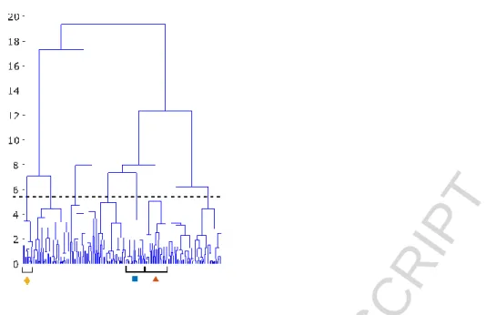
to be associated with their effect on the objectives. For the clay soil, hierarchical clustering was used
to divide the sets of management actions into 9 clusters (Fig 3). Looking at the mean of the
profitability objective in the clusters, three profitable strategies were identified:
1. Applying no FYM and relatively high fertiliser N over 3 applications
2. Applying a little FYM and a slightly less N fertiliser over 2 applications
3. Applying much FYM and rather less N fertiliser over 2 applications
Notably, in these strategies, fertiliser applications tended to start later (from the 4th possible
application date) than other less-profitable strategies (Supplementary Information, Fig S2). The first
two strategies were associated with high yield, whilst for the third profitable strategy the yield was
slightly less and the profitability arose from lower fertiliser costs. FYM application was,
unsurprisingly, associated with increases in SOC. Most of the profitable strategies were associated
ACCEPTED MANUSCRIPT
14
of N fertiliser were applied). Also, in the clay soil the maximum yield was higher than the sandy clay
and sandy loam soils.
Figure 1: Trade-off frontiers (a-f) and cluster characteristics (g-r) in clay soil. Units are: Yield (t/ha),
Profitability (x103 £ / ha /year), N2O ( x103 CO2 equivalent yr-1), change in SOC - δSOC (%). Note that
for N2O, increasing values are shown from right to left or top to bottom because this objective was
minimised in the optimisation process. This means that, consistently across the plots, trade-offs
show trends from the top left to the bottom right of the plots and synergies trends from the bottom
left to the top right. Points within the most profitable clusters are highlighted; all other points are
shown as small grey circles. Histograms of the cluster variates show the fraction of the points in each
cluster with a particular management value, where n is the number of management strategies (i.e.
points) in each cluster, N Fert is the total N applied in fertiliser, First N is the week of the first N
application, # Apps is the number of fertiliser applications and FYM is the amount of farm yard
ACCEPTED MANUSCRIPT
15
Figure 2: Trade off frontiers between the objectives relating to nitrogen cycling for the clay soil.
Units are: N2O ( x10 3
CO2 equivalent yr -1
), N surplus (kg ha-1 yr-1), NUE (-). Yellow diamonds, red
triangle and blue squares indicate points in the frontier that correspond to the clusters detailed in
Fig. 1, g-r grey dots show all other points in the frontier. Note that for N2O and N surplus, increasing
values are shown from right to left or top to bottom because these objectives were minimised in the
optimization process. This means that, consistently across the plots, trade-offs show trends from the
ACCEPTED MANUSCRIPT
16
Figure 3: Hierarchical cluster results for clay soil, with the profitable clusters highlighted. The dotted
line indicates the division of the dataset into 9 clusters.
In the sandy clay soil the same trade-offs and synergies between objectives were observed as in the
clay soil (Fig 4a-f). Two profitable management strategies were identified (Fig 4g-n):
1. High application of FYM, 1-3 applications of a small amount of N fertiliser
2. Low or Medium application of FYM, 1-3 applications of a medium amount of N fertiliser
In this soil, most of the points in the optimal set were high yielding (Fig 4f). Profitable strategies were
ACCEPTED MANUSCRIPT
17
Figure 4: Trade-off frontiers (1-f) and cluster characteristics (g-r) in sandy clay soil. Units are: Yield
(t/ha), Profitability (x103 £ / ha / year), N2O ( x103 CO2 equivalent), Change in SOC - δSOC (%). Note
that for N2O, increasing values are shown from right to left or top to bottom because this objective
was minimised in the optimisation process. This means that, consistently across the plots, trade-offs
show trends from the top left to the bottom right of the plots and synergies trends from the bottom
left to the top right. Points within the most profitable clusters are highlighted; all other points are
shown as small grey circles. Histograms of the cluster variates show the fraction of the points in each
cluster with a particular management value, where n is the number of management strategies (i.e.
points) in each cluster, N Fert is the total N applied in fertiliser, First N is the week of the first N
application, # Apps is the number of fertiliser applications and FYM is the amount of farm yard
manure applied.
For the sandy loam soil (Fig. 5), the highest possible profitability was £390 ha-1 yr-1, lower than the
sandy clay and clay soils (£458 and £624 ha-1 yr-1 respectively). Meanwhile, the maximum possible
yield 7.5 t ha-1 for the sandy loam soil, was higher than possible for the sand clay (7.0 t ha-1) but
lower than for the clay soil (8.7 t ha-1).
ACCEPTED MANUSCRIPT
18
1. High FYM, high N fertiliser in 2-3 applications, starting early
2. High FYM, medium N fertiliser, typically 2-3 applications, starting slightly later
3. No FYM, medium N fertiliser, typically 3-4 applications, starting even later
Figure 5: Trade-off frontiers (1-f) and cluster characteristics (g-r) in sandy loam soil. Units are: Yield
(t/ha), Profitability (x103 £ / ha / year), N
2O ( x103 CO2 equivalent), Change in SOC - δSOC (%). Note
that for N2O, increasing values are shown from right to left or top to bottom because this objective
was minimised in the optimisation process. This means that, consistently across the plots, trade-offs
show trends from the top left to the bottom right of the plots and synergies trends from the bottom
left to the top right. Points within the most profitable clusters are highlighted; all other points are
shown as small grey circles. Histograms of the cluster variates show the fraction of the points in each
cluster with a particular management value, where n is the number of management strategies (i.e.
points) in each cluster, N Fert is the total N applied in fertiliser, First N is the week of the first N
application, # Apps is the number of fertiliser applications and FYM is the amount of farm yard
ACCEPTED MANUSCRIPT
19
Combining the objectives across three fields of equal area but differing in soil texture (clay, sandy
clay, sandy loam) led to a combined trade-off frontier (Fig. 6). Notably, for the combined
management, it becomes more clear that the frontier is a multi-dimensional surface with the Pareto
optimal points more spread out compared to the management for each of the soils individually (Figs.
1, 4 and 5). The relationship between the profitability and N2O emissions was synergistic for high
emissions, but becomes a trade-off at lower emissions. This change at the frontier, from synergy to
trade-off, was clearer than in the individual soils and indicated that a reduction in nitrous oxide
emissions beyond a certain point would be associated with a large reduction in profitability (Fig. 6e).
Multiple profitable strategies perform similarly with respect to multiple objectives (e.g. green and
yellow clusters in Fig. 6) meaning that there is freedom to make choices between these strategies
based on additional objectives not captured by the model. The most profitable strategies (the blue
cluster in Fig. 6) produced lower nitrous oxide emissions than the other profitable clusters, all of
which resulted in an increase in SOC.
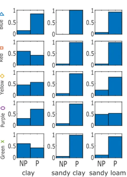
Interestingly, all of the more profitable clusters in the combined management included the most
profitable management strategies for the sandy clay soil, which had the lowest maximum yield (Fig.
8). Furthermore, only one of the five management strategies on the sandy loam soil (which had the
medium maximum yield) included less profitable management strategies on this soil. On the clay soil
(which had the highest maximum yield), there were a wider range of management strategies that
resulted in profitable overall management. Compared to the strategies identified for the clay soil
alone (Fig 1.), the strategies that were profitable on clay in the case of combined management
included more in which manure was applied to the clay soil, and more numerous fertiliser
applications (Fig. 7).
This shift to less profitable strategies occurs in the clay soil but not in the sandy clay when combined
management is considered. The reasons for this are complex but occur because of the effect that a
ACCEPTED MANUSCRIPT
20
clay soil, most of the possible reduction in N2O emissions can be achieved whilst remaining
profitable (i.e. the frontier has a fairly straight vertical edge in Fig. 4e). In the clay soil however, there
is a discernible trade-off that emerges to reach the lowest possible emissions (i.e. the top edge of
the frontier is more rounded in Fig. 1e). Additionally, in the clay soil the differences between
profitability of the more profitable strategies was smaller than in the sandy clay soil (i.e. with respect
to profitability, the points are grouped together predominantly in the high profitability region for the
clay soil – Fig. 1, but are more spread out for the sandy clay soil – Fig. 4). This means that, to
maintain overall profitability for a decrease in the profitability in the sandy clay soil, a relatively large
increase in profitability on another soil would be necessary. Hence optimal combined strategies
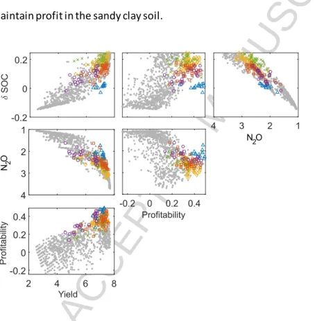
maintain profit in the sandy clay soil.
Figure 6: Trade-off frontiers when managing three fields each of equal area but each of a different
soil texture (clay, sandy clay, sandy loam). Units are: Yield (t/ha), Profitability (x103 £ / ha / year), N2O
( x103 CO2 equivalent), Change in SOC - δSOC (%). Note that for N2O, increasing values are shown
from right to left or top to bottom because this objective was minimised in the optimisation process.
ACCEPTED MANUSCRIPT
21
bottom right of the plots and synergies trends from the bottom left to the top right. Points within
the most profitable clusters are highlighted; all other points are shown as small grey circles.
Histograms of the cluster characteristics for the most profitable clusters are shown in Fig. 7.
Figure 7: Characteristics of the profitable clusters for the combined management of three soil types.
Histograms of the cluster variates show the fraction of the points in each cluster with a particular
management value, where n is the number of management strategies (i.e. points) in each cluster, N
Fert is the total N applied in fertiliser, First N is the week of the first N application, # Apps is the
ACCEPTED MANUSCRIPT
22
Figure 8: Proportion of the points within each cluster that correspond to profitable management of
that soil type. On the x-axis, P corresponds to profitable and NP to not profitable. Profitable points
are defined as the 30% of most profitable points for that soil type.
Discussion
Trade-offs between objectives
One distinctive feature of the results is the non-linearity of the trade-off between yield and N2O
emissions. This is not unexpected as high yields are associated with high N application, either in the
form of fertiliser or manure, but is important to note because many national greenhouse gas
inventories follow an emissions factor approach that effectively assumes this relationship is linear
(Eggleston et al., 2006; Shcherbak et al., 2014).. Recent work has suggested that the increase in N2O
emissions with increasing N application is non-linear (Shcherbak et al., 2014), and here, when the
trade-off is considered with respect to yield, this non-linearity is exacerbated as at high N application
further increases in N applied result in only a marginal increase in yield. Linquist et al. (2012)
considered the trade-off between greenhouse gas and cereal crop production. They concluded that
ACCEPTED MANUSCRIPT
23
is comparable to the point at which we observed the non-linear increase in GHG production (90% of
the maximum yield in the clay soil, 85% in the sandy clay and 88% in the sandy loam soil). A similar
finding was also reported by Nguyen et al., (2018) who suggested that 90% of potential production
can be achieved with minimal impacts, including greenhouse gas emissions. It is interesting to note
that this non-linear point is comparable to the 80% of potential yield that is often considered as the
‘exploitable yield’ in yield gap analysis (Lobell et al., 2009; van Ittersum et al., 2013). Whilst this
exploitable yield has been reached from a resource use and profitability persp ective, in our analysis
is corresponds more to the threshold that limits a negative environmental impact, as some of these
high emission management strategies still appear to be profitable in our analysis.
The results also highlight a trade-off between N2O emissions and increasing SOC in the soil. This is in
part due to the control options by which the SOC can be increased in the simulations; either by
manure addition or by increasing N application in such a way that yield increased and hence crop
residues also. Both mechanisms are typically associated with an increase in N2O emissions. Bos et al.
(2017) showed that net GHG emission reductions could not be obtained with manure application,
and only the application of compost resulted in larger emission reductions because of SOC increase
compared to N20 emission increase. There are also indications that N2O emissions may be inherently
higher from soils with higher SOC (Palmer et al., 2017; Charles et al., 2017), as this would reduce the
chance that N2O emissions are limited by C availability in soil (Charles et al., 2017). Other studies,
however, have not found a significant effect of SOC (Buckingham et al., 2014). When considering
carbon sequestration to mitigate GHG production, the net effect of sequestration and emissions
must be considered. Other studies have also suggested that, in terms of global warming potential
carbon sequestration may be offset by N2O emissions (Powlson et al. 2011; Zhou et al., 2017). A
systems perspective is also clearly necessary as, if manure was not applied to the soil, it would still
ACCEPTED MANUSCRIPT
24
for other reasons such as increasing future soil fertility (Garratt et al., 2018) and reducing erosion
risk.
The EU nitrogen panel has made recommendations for NUE and N surplus (EU Nitrogen Expert
Panel., 2015), suggesting a range of NUE from 0.5 - 0.9 combined with an N surplus of less than 80 kg
ha-1 yr-1. In our study these ranges were met by using strategies in which very little manure was
applied, for example the blue square cluster (Fig. 2) in which no manure was applied or very few of
the red triangle cluster in which a small amount of manure was applied. This corresponds to the fact
that manure applications were associated with an increase in N2O emissions in the simulations, and
also with increased N leaching. Some thought must be given to how NUE and N surplus is calculated
when applying organic matter to the soil, as nitrogen applied in one year may benefit crops in future
years. For this reason N inputs and outputs were calculated for the whole simulation , however,
there was also likely a build up of soil nitrogen in this period. Indeed, an increase in SOC would
require this (Van Groenigen et al., 2017); So if increasing SOC is an objective, the NUE and N surplus
targets or calculation approaches may need to be reconsidered concurrently.
Management across soil types
As expected, the model simulated differences between the soils in terms of the yield and N2O
emissions. The N2O emissions from the sandy loam soil were notably less than from the other two
soils, particularly at greater N application rates. This corresponds to the findings from other studies
which suggest that emissions from fine textured soils are greater than from coarse textures (Charles
et al., 2017) and that water filled pore space is a key factor affecting emissions ( García‐Marco et al.,
2014). Thus soils which retained more water, emitted more N2O. The lower NUE values and higher N
surplus values in this soil also suggest that more N is lost from the soil profile by leaching, as would
ACCEPTED MANUSCRIPT
25
Interestingly, the maximum possible increase in SOC was comparable for all three soils. The
simulated potential is of course related to the initial SOC in the simulations. In this case, the
simulations were based on soils under long-term arable management with low initial SOC and in this
situation it seems that, for the soil textures we considered, the soil texture had little effect on the
possible increase in SOC.
In general, profitable strategies were associated with large yields. At the highest yields, we might
have expected to see a trade-off between these two objectives; indeed, in yield gap analysis, 80% of
the potential yield is considered as the ‘exploitable yield’ (Lobell et al., 2009; van Ittersum et al.,
2013), representing a point at which there starts to be a trade-off between the two objectives
because the cost of inputs outweighs the increase in sale price due to the increase in yield. Here,
however, as in other studies (Silva et al., 2017), we did not observe this trade -off. Nevertheless, in
the clay soil, a reduction of yield to around 70% of the maximum could be achieved with very little
impact on the profitability (Fig. 1). In the sandy clay, reductions in yield resulted in a linear reduction
in profitability (Fig. 4). In both case, strategies that reduced yield but maintained profitability were
associated with large manure application rates and small amounts of N fertiliser. This strategy was
not identified as a possibility in the sandy clay soil, which also had the l owest yield potential. In this
soil, all the profitable strategies were associated with high yields. This suggests that there is less
opportunity to adapt management strategies whilst remaining profitable.
On many farms, such as those in the UK, different soil types are present and these soils must be
managed simultaneously. Considering the combined options across these different soils means that
additional strategies can be identified to deliver the same objectives overall. Here, for example, the
clay soil could be managed in a way that was not necessarily the most profitable for that soil, but
contributed to improving the other objectives. The loss in the likely profit from this soil could then
ACCEPTED MANUSCRIPT
26
One ongoing debate regarding sustainable agriculture relates to the notion of sharing or sparing land
in agricultural production (Phalan et al., 2011; Fischer et al., 2014). This relates to considering
whether environmental objectives might be best achieved by reducing production (and thus
negative environmental impacts) across all agricultural land (sharing) or whether it would be
preferable to remove some agricultural land from production entirely and use remaining agricultural
land even more intensively (sparing). Most research in this area has focussed on the trade-off
between biodiversity and production. However, recent studies suggest that land-sparing might help
mitigate leaching and GHG emissions as well (Lamb et al., 2016; Balmford et al., 2018).
Generally, for land sparing it might be expected that the least productive agricultural land be
removed from production because the focus is on yield and profit. Contrary to this, however, the
results here suggest that it is management of the most productive soil that should be targeted to
improve the multi-objective performance. Biodiversity is not a part of this analysis, nor is carbon
sequestration in spared land. In this study, land cannot be entirely removed from production in the
way the control variables in this study have been implemented, and the environmental objectives
focus mainly on nitrogen. However, given the typical nitrogen response curve of crops, it is
unsurprising that spreading nitrogen thinly over a larger area will be preferable to putting the same
amount on a smaller area. This takes advantage of the larger yield increase per unit nitrogen that
occurs at low application rates compared to those that occur at higher application rates. This means,
however, that in a land sparing scenario, the agricultural land that is managed more intensively is
likely to result in higher nitrous oxide emissions per unit yield. A natural extension of this work
would therefore be to include biodiversity objectives within the optimization. Any trade-off between
these objectives and nitrogen cycling objectives should then become apparent.
Envisioning future landscapes
One core aim of this paper is to illustrate the potential of of this approach to identify possibilities for
ACCEPTED MANUSCRIPT
27
possibilities, the intention being that these can be presented to and discussed with stakeholders.
Specifically, this approach could be used as a tool within a visioning and backcasting exercise (i.e.
envisioning the future and then working backwards from this vision until the current state is
reached). Visioning and backcasting is an approach that was developed in the energy sector as a tool
to identify transformation pathways (Robinson, 1982) and has subsequently been used in other
sectors as a tool for considering transformative change within complex systems (Dreborg, 1996;
Vergragt and Quist, 2011). The first step is to envisage a desirable future and this is often done using
a participatory that brings together multiple stakeholders with different perspectives. The idea in the
visioning step is to focus on the key factors that are important to the different stakeholders for the
future, rather than discussing the current problems and barriers to change (as can easily happen in a
forecasting approach, or when the current situation is the focus of discussion). Gil et al. (2018)
represent an example, where priorities for SDG-2 (‘End Hunger’) were set by comparing SDG-2
indicator target values for 2030 with current values. With the end vision in sight, the backcasting
process then allows stakeholders to be more creative in considering how any barriers might be
overcome. Thus, in theory, the approach should allow more room for a truly transformative pathway
to be identified.
Such approaches encourage idealism, the philosophy being that our visions provide the motivation
to develop new approaches and therefore reshape what is possible (Wright, 2010). Yet this idealism
must be balanced with realism in order to generate visions that are also plausible and tangible so
that action can be taken (Wiek and Iwaniec, 2014). Without this, there is a risk that an idealistic
future vision may include multiple objectives that are not physically possible to achieve concurrently.
Trade-off frontiers identified by multi-objective algorithms could therefore be used as a tool to
encourage stakeholders to discuss trade-offs whilst they are developing this future vision. This would
allow challenging discussions about trade-offs to occur during the visioning process, rather than
ACCEPTED MANUSCRIPT
28
system and more focus on what would be desirable in future. For instance, the example presented in
this study could be used to inform stakeholder discussion about the relative importance of
minimising nitrous oxide emissions from soil compared to maximising yield, without the idealistic
assumption that both can be achieved simultaneously and without apportioning blame with regards
to the current state of the system.
In this example the focus was on wheat production in a small landscape and with a defined set of
control variables relating to fertiliser and manure application. Thus, there is clearly scope to expand
the method to consider more diverse agricultural practices in more complex landscapes as the scale
and context will affect the trade-offs that can be achieved. These could include practices that are of
interest to stakeholders within a particular context and things that are technically possible and the
scales (field, farm, region) at which different options could be implemented. Even so, the approach
highlighted the range of possibilities that might be achievable with simple changes and the
opportunities in considering the heterogeneity of the landscape.
There are various technical challenges in the optimization approach, including the risk of the
algorithm becoming stuck in local minima and the inconvenience of the algorithm converging slowly
because extreme control variables are selected and are difficult to simulate . These risks would be
even more present in more complex modelling scenarios considering more complex landscapes and
management possibilities. However, we found that seeding some of the initial population with a
number of likely scenarios was effective at reducing the number of steps needed for convergence,
an approach that has been useful elsewhere (Milne et al., in review). Within the initial population,
several possible fertiliser applications were set to a rate of zero. When using more complex sets of
control variables, subgroups of these control could be optimised initially in order to be able to seed
optimization of the complete set.
The cluster analysis was used as a tool to relate the control variables to the resulting sets of
ACCEPTED MANUSCRIPT
29
Pareto front. It is particularly interesting that for some pairs of objectives similar trade -offs can be
achieved by alternative strategies (e.g. those from different clusters). For example, similar yields and
GHG emissions occur for strategies identified by the clusters of red squares and green crosses in Fig.
6. In this case, more points occur in the red square cluster and fewer in green cross cluster. In
general, the points in the green cross cluster dominate those in the red square cluster with respect
to the indicators of SOC. Without this dominance in another factor, it is likely that this management
strategy would occur less frequently in the population. Indeed, if the algorithm were optimised
based on yield and GHG objectives alone it may even be overlooked entirely, if a strategy from the
red square cluster marginally outperforms the strategy of the green cross cluster. Thus inclusion of
another objective enabled the identification of an alternative management approach with similar
performance for another objective.
To capture the complexity and the multiple stakeholder objectives and to identify a diverse range of
strategies, it may seem desirable to include more objectives. However, with more objectives it
becomes increasingly difficult to visualise the results and communicate them clearly. Additionally,
models are unlikely to be able to simulate all of stakeholders’ priorities. We suggest, therefore, that
the objectives simulated and optimised by the model are viewed as a subset of the stakeholders’
priorities. In this case the objectives used in the model were a subset of those identified by Gil et al.
(2018) which included NUE, N surplus and greenhouse gas emissions intensity as priorities for
agriculture in the Netherlands as well as pesticide use and genetic diversity which cannot currently
be represented in the model. In most situations there will also exist additional objectives that have
not been quantified by the model which stakeholders will be considering when they interpret the
results. For each management strategy, another analysis exercise (e.g. a participatory method with
the stakeholders or empirical evidence) could then be used to identify how the management
strategies would likely affect unmodelled objectives. However, there may also be distinct
ACCEPTED MANUSCRIPT
30
neglected by the optimization algorithm. Although it is likely to increase convergence time, future
algorithms should retain solutions that are ‘almost’ optimal within a chosen tolerance, particularly if
they are associated with distinctly different management strategies. Given complex control
variables, this should increase the number of distinct management strategies that might be of
interest for stakeholder discussion and might meet other, untested objectives such as those relating
to biodiversity.
Acknowledgements
Rothamsted Research receives grant aided support from the Biotechnology and Biological Sciences
Research Council (BBSRC) of the United Kingdom. This research was funded by a DEFRA and EU
collaborative project “Targets for Sustainable And Resilient Agriculture” (TSARA), received as part of
the FACCE-JPI Surplus initiative, the Biotechnology and Biological Sciences Research Council (BBSRC)
Institute Strategic Programme (ISP) grants, “Soils to Nutrition” (S2N) grant number
BBS/E/C/000I0330, and the joint Natural Environment Research Council (NERC) and the
Biotechnology and Biological Sciences Research Council (BBSRC) ISP grant “Achieving Sustainable
Agricultural Systems” (ASSIST) grant number NE/N018125/1 LTS-M ASSIST, using facilities funded by
the BBSRC.
References
1. Balmford, A., Amano, T., Bartlett, H., Chadwick, D., Collins, A., Edwards, D., Field, R.,
Garnsworthy, P., Green, R., Smith, P., Waters, H., Whitmore A., Broom,D., Chara, J., Finch, T.,
Garnett, E., Gathorne-Hardy, A., Hernandez-Medrano, J., Herrero, M., Hua, F., Latawiec, A.,
ACCEPTED MANUSCRIPT
31
(2018) The environmental costs and benefits of high-yield farming, Nature Sustainability 1,
477-485 doi: 10.1038/s41893-018-0138-5
2. Bos, J.F., ten Berge, H.F., Verhagen, J. and van Ittersum, M.K. (2017). Trade-offs in soil fertility
management on arable farms. Agricultural Systems, 157, pp.292-302. Doi:
10.1016/j.agsy.2016.09.013
3. Buckingham, S., Anthony, S., Bellamy, P.H., Cardenas, L.M., Higgins, S., McGeough, K. and Topp,
C.F.E. (2014). Review and analysis of global agricultural N2O emissions rele vant to the UK.
Science of the Total Environment, 487.
4. Burns, F., Eaton, M.A., Barlow, K.E., Beckmann, B.C., Brereton, T., Brooks, D.R., Brown, P.M., Al
Fulaij, N., Gent, T., Henderson, I. and Noble, D.G. (2016). Agricultural management and climatic
change are the major drivers of biodiversity change in the UK. PLoS One, 11(3), p.e0151595.
5. Campbell, B., Beare, D., Bennett, E., Hall-Spencer, J., Ingram, J., Jaramillo, F., Ortiz, R.,
Ramankutty, N., Sayer, J. and Shindell, D. (2017). Agriculture production as a major driver of the
Earth system exceeding planetary boundaries. Ecology and Society, 22(4).
6. Cao, K., Batty, M., Huang, B., Liu, Y., Yu, L., & Chen, J. (2011). Spatial multi -objective land use
optimization: extensions to the non-dominated sorting genetic algorithm-II. International Journal
of Geographical Information Science, 25(12), 1949-1969. Doi:
10.1016/j.compenvurbsys.2011.08.001
7. Charles, A., Rochette, P., Whalen, J.K., Angers, D.A., Chantigny, M.H. and Bertrand, N. (2017).
Global nitrous oxide emission factors from agricultural soils after addition of organic
amendments: A meta-analysis. Agriculture, Ecosystems & Environment, 236, pp.88-98. Doi:
10.1016/j.agee.2016.11.021
8. Coleman, K., Muhammed, S. E., Milne, A. E., Todman, L. C., Dailey, A. G., Glendining, M. J., &
Whitmore, A. P. (2017). The landscape model: A model for exploring trade -offs between
ACCEPTED MANUSCRIPT
32
9. Deb K, Pratap A, Agarwal S, Meyarivan T. (2002). A fast and elitist multiobjective genetic
algorithm: NSGA-II. Transactions on Evolutionary Computation 6:182–197.
10. Dreborg, K.H., 1996. Essence of backcasting. Futures, 28(9), pp.813-828.
11. Eggleston, S., Buendia, L., Miwa, K., Ngara, T. and Tanabe, K. (2006). IPCC guidelines for national
greenhouse gas inventories (Vol. 4). Hayama, Japan: Institute for Global Environmental
Strategies (IGES).
12. Estes, L. D., Searchinger, T., Spiegel, M., Tian, D., Sichinga, S., Mwale, et al. (2016). Reconciling
agriculture, carbon and biodiversity in a savannah transformation frontier. Phil. Trans. R. Soc. B,
371(1703), 20150316. Doi: 10.1098/rstb.2015.0316
13. EU Nitrogen Expert Panel. (2015). Nitrogen Use Efficiency (NUE) an indicator for the utilization of
nitrogen in food systems. Wageningen University, Alterra, Wageningen, Netherlands.
14. Fischer, J., Abson, D.J., Butsic, V., Chappell, M.J., Ekroos, J., Hanspach, J., Kuemmerle, T., Smith,
H.G. and von Wehrden, H. (2014). Land sparing versus land sharing: moving forward.
Conservation Letters, 7(3), pp.149-157.
15. García‐Marco, S., Ravella, S. R., Chadwick, D., Vallejo, A., Gregory, A. S., & Cárdenas, L. M. (2014).
Ranking factors affecting emissions of GHG from incubated agricultural soils. European journal of
soil science, 65(4), 573-583.
16. Garratt, M.P., Bommarco, R., Kleijn, D., Martin, E., Mortimer, S.R., Redlich, S., Senapathi, D.,
Steffan-Dewenter, I., Świtek, S., Takács, V. and van Gils, S. (2018). Enhancing Soil Organic Matter
as a Route to the Ecological Intensification of European Arable Systems. Ecosystems
17. Gil, J.D.B., Reidsma, P., Giller, K., Todman, L., Whitmore, A. and van Ittersum, M. (2018).
Sustainable development goal 2: Improved targets and indicators for agriculture and food
security. Ambio, pp.1-14.
18. Groot, J. C., Rossing, W. A., Jellema, A., Stobbelaar, D. J., Renting, H., & Van Ittersum, M. K.
ACCEPTED MANUSCRIPT
33
landscape quality—a methodology to support discussions on land-use perspectives. Agriculture,
Ecosystems & Environment, 120(1), 58-69. Doi: 10.1016/j.agee.2006.03.037
19. Groot, J.C., Oomen, G.J. and Rossing, W.A. (2012). Multi-objective optimization and design of
farming systems. Agricultural Systems, 110. Doi: 10.1016/j.agsy.2012.03.012
20. Groot, J.C., Yalew, S.G. and Rossing, W.A. (2018). Exploring ecosystem services trade-offs in
agricultural landscapes with a multi-objective programming approach. Landscape and Urban
Planning, 172, pp.29-36.
21. Hou, Y., Velthof, G.L. and Oenema, O. (2015). Mitigation of ammonia, nitrous oxide and methane
emissions from manure management chains: a meta‐analysis and integrated assessment. Global
change biology, 21(3), pp.1293-1312. Doi: 10.1111/gcb.12767
22. Hu, H., Fu, B., Lü, Y., & Zheng, Z. (2015). SAORES: a spatially explicit assessment and optimization
tool for regional ecosystem services. Landscape ecology, 30(3), 547-560. Doi:
10.1007/s10980-014-0126-8
23. Huang, K., Liu, X., Li, X., Liang, J., & He, S. (2013). An improved artificial immune system for
seeking the Pareto front of land-use allocation problem in large areas. International Journal of
Geographical Information Science, 27(5), 922-946. Doi: 10.1080/13658816.2012.730147
24. Ibrahim, A., Rahnamayan, S., Martin, M.V. and Deb, K. (2016), July. 3D-RadVis: Visualization of
Pareto front in many-objective optimization. In 2016 IEEE Congress on Evolutionary Computation
(CEC). IEEE. Doi: 10.1109/CEC.2016.7743865
25. Kanter, D.R., Musumba, M., Wood, S.L., Palm, C., Antle, J., Balvanera, P., Dale, V.H., Havlik, P.,
Kline, K.L., Scholes, R.J. and Thornton, P. (2018). Evaluating agricultural trade-offs in the age of
sustainable development. Agricultural Systems, 163. Doi: 10.1016/j.agsy.2016.09.010
26. Kennedy, C. M., Hawthorne, P. L., Miteva, D. A., Baumgarten, L., Sochi, K., Matsumoto, M., ... &
Develey, P. F. (2016). Optimizing land use decision-making to sustain Brazilian agricultural
profits, biodiversity and ecosystem services. Biological Conservation, 204, 221-230. Doi:
ACCEPTED MANUSCRIPT
34
27. Klapwijk, C.J., Van Wijk, M.T., Rosenstock, T.S., van Asten, P.J., Thornton, P.K. and Giller, K.E.
(2014). Analysis of trade-offs in agricultural systems: current status and way forward. Current
opinion in Environmental sustainability, 6. Doi: 10.1016/j.cosust.2013.11.012
28. Lamb, A., Green, R., Bateman, I., Broadmeadow, M., Bruce, T., Burney, J., Carey, P., Chadwick, D.,
Crane, E., Field, R. and Goulding, K. (2016). The potential for land sparing to offset greenhouse
gas emissions from agriculture. Nature Climate Change, 6(5).
29. Lautenbach, S., Volk, M., Strauch, M., Whittaker, G. and Seppelt, R. (2013). Optimization-based
trade-off analysis of biodiesel crop production for managing an agricultural catchment.
Environmental Modelling & Software, 48, pp.98-112.
30. Linquist, B., Van Groenigen, K.J., Adviento‐Borbe, M.A., Pittelkow, C. and Van Kessel, C. (2012).
An agronomic assessment of greenhouse gas emissions from major cereal crops. Global Change
Biology, 18. Doi: 10.1111/j.1365-2486.2011.02502.x
31. Lobell, D.B., Cassman, K.G. and Field, C.B. (2009). Crop yield gaps: their importance, magnitudes,
and causes. Annual review of environment and resources, 34, pp.179-204.
32. MATLAB and Statistics Toolbox Release 2018a, The MathWorks, Inc., Natick, Massachusetts,
United States.
33. Milne, A.E., Coleman, K., Todman, L.C., Whitmore, A.P. (in review). Accounting for landscape
interactions in multi-objective optimization of ecosystem services. Environmental Monitoring
and Assessment.
34. Nassauer, J.I. and Corry, R.C. (2004). Using normative scenarios in landscape ecology. Landscape
ecology, 19(4). Doi: 10.1023/B:LAND.0000030666.55372.ae
35. Nguyen, T.H., Cook, M., Field, J.L., Khuc, Q.V. and Paustian, K. (2018). High-resolution trade-off
analysis and optimization of ecosystem services and disservices in agricultural landscapes.
Environmental modelling & software, 107, pp.105-118. Doi: 10.1016/j.envsoft.2018.06.006
36. Palmer, J., Thorburn, P.J., Biggs, J.S., Dominati, E.J., Probert, M.E., Meier, E.A., Huth, N.I., Dodd,
ACCEPTED MANUSCRIPT
35
carbon contributes both positively and negatively to ecosystem services in wheat
agro-ecosystems. Frontiers in plant science, 8, p.731. doi: 10.3389/fpls.2017.00731
37. Phalan, B., Onial, M., Balmford, A. and Green, R.E. (2011). Reconciling food production and
biodiversity conservation: land sharing and land sparing compared. Science, 333(6047),
pp.1289-1291.
38. Polasky, S., Nelson, E., Camm, J., Csuti, B., Fackler, P., Lonsdorf, E., ... & Haight, R. (2008). Where
to put things? Spatial land management to sustain biodiversity and economic returns. Biological
conservation, 141(6), 1505-1524. Doi: 10.1016/j.biocon.2008.03.022
39. Powlson, D. S., Whitmore, A. P., & Goulding, K. W. T. (2011). Soil carbon sequestration to
mitigate climate change: a critical re‐examination to identify the true and the false. European
Journal of Soil Science, 62(1), 42-55.
40. Robinson, J. B. (1982). Energy backcasting A proposed method of policy analysis. Energy policy,
10(4), 337-344. Doi: 10.1016/0301-4215(82)90048-9
41. Schönhart, M., Schauppenlehner, T., Schmid, E. and Muhar, A. (2011). Integration of bio-physical
and economic models to analyze management intensity and landscape structure effects at farm
and landscape level. Agricultural Systems, 104. Doi: 10.1016/j.agsy.2010.03.014
42. Schönhart, M., Schauppenlehner, T., Kuttner, M., Kirchner, M. and Schmid, E. (2016). Climate
change impacts on farm production, landscape appearance, and the environment: Policy
scenario results from an integrated field-farm-landscape model in Austria. Agricultural Systems,
145. Doi: 10.1016/j.agsy.2016.02.008
43. Shcherbak, I., Millar, N. and Robertson, G.P. (2014). Global metaanalysis of the nonlinear
response of soil nitrous oxide (N2O) emissions to fertilizer nitrogen. Proceedings of the Nationa l
Academy of Sciences, 111. Doi: 10.1073/pnas.1322434111
44.
Silva, J.V., Reidsma, P. and van Ittersum, M.K. (2017). Yield gaps in Dutch arable farming systems:ACCEPTED MANUSCRIPT
36
45. Steffen, W., Richardson, K., Rockström, J., Cornell, S.E., Fetzer, I., Bennett, E.M., Biggs, R.,
Carpenter, S.R., De Vries, W., De Wit, C.A. and Folke, C. (2015). Planetary boundaries: Guiding
human development on a changing planet. Science, 347(6223), p.1259855.
46. Storn R, Price K. (1997). Differential Evolution – A Simple and Efficient Heuristic for global
Optimization over Continuous Spaces. Journal of Global Optimization 11:341–359.
47. Tušar, T. and Filipič, B. (2015). Visualization of Pareto front approximations in evolutionary
multiobjective optimization: A critical review and the prosection method. IEEE Transactions on
Evolutionary Computation, 19(2). Doi: 10.1109/TEVC.2014.2313407
48. Van Groenigen, J.W., Van Kessel, C., Hungate, B.A., Oenema, O., Powlson, D.S. and Van
Groenigen, K.J. (2017). Sequestering soil organic carbon: a nitrogen dilemma.
49. Van Ittersum, M.K., Ewert, F., Heckelei, T., Wery, J., Olsson, J.A., Andersen, E., Bezlepkina, I.,
Brouwer, F., Donatelli, M., Flichman, G. and Olsson, L. (2008). Integrated assessment of
agricultural systems–A component-based framework for the European Union (SEAMLESS).
Agricultural systems, 96. Doi: 10.1016/j.agsy.2007.07.009
50. van Ittersum, M.K., Cassman, K.G., Grassini, P., Wolf, J., Tittonell, P. and Hochman, Z. (2013).
Yield gap analysis with local to global relevance—a review. Field Crops Research, 143, pp.4-17.
51. Ward, J. H. Jr. Hierarchical grouping to optimize an objective function (1963). Journal of the
America Statistical Association. 58, 236–244, Doi: 10.2307/2282967.
52. Wiek, A., & Iwaniec, D. (2014). Quality criteria for visions and visioning in sustainability science.
Sustainability