Article
A Software Reliability Model with a Weibull Fault
Detection Rate Function Subject to Operating
Environments
Kwang Yoon Song 1, In Hong Chang 1,* and Hoang Pham 2
1 Department of Computer Science and Statistics, Chosun University, 309 Pilmun-daero Dong-gu, Gwangju, 61452, Korea; [email protected] (K.Y.S.)
2 Department of Industrial and Systems Engineering, Rutgers University, 96 Frelinghuysen Road, Piscataway, NJ 08855-8018, USA; [email protected]
* Correspondence: [email protected]; Tel.: +82-62-220-6621
ABSTRACT: The main focus when developing software is to improve the reliability and stability of a software system. When software systems are introduced, these systems are used in field environments that are the same as or close to those used in the development-testing environment; however, they may also be used in many different locations that may differ from the environment in which they were developed and tested. In this paper, we propose a new software reliability model that takes into account the uncertainty of operating environments. The explicit mean value function solution for the proposed model is presented. Examples are presented to illustrate the goodness-of-fit of the proposed model and several existing non-homogeneous Poisson process (NHPP) models and confidence intervals of all models based on two sets of failure data collected from software applications. The results show that the proposed model fits the data more closely than other existing NHPP models to a significant extent.
Keywords: non-homogeneous poisson process, software reliability; weibull function; mean squared error
1. Introduction
Chatterjee and Singh [5] proposed a software reliability model based on NHPP that incorporates a logistic–exponential testing coverage function with imperfect debugging. In addition, Chatterjee and Shukla [6] developed a software reliability model that considers different types of faults incorporating both imperfect debugging and a change point. Generally, existing models are applied to software testing data and then used to make predictions on the software failures and reliability in the field. Here, the important point is that the test environment and operational environment are different from each other. Once software systems are introduced, the software systems used in the field environments are the same as or close to those used in the development-testing environment; however, the systems may be used in many different locations. Several researchers started applying the factor of operational environments. A few researchers, Yang and Xie, Huang et al., and Zhang et al. [7-9], proposed a method of predicting the fault detection rate to reflect changes in operating environments, and used methodology that modifies the software reliability model in the operating environments by introducing a calibration factor. Teng and Pham [10] discussed a generalized model that captures the uncertainty of the environment and its effects upon the software failure rate. Pham [11-12] and Chang et al. [13] developed a software reliability model incorporating the uncertainty of the system fault-detection rate per unit of time subject to the operating environment. Honda et al. [14] proposed a generalized software reliability model (GSRM) based on a stochastic process and simulated developments that include uncertainties and dynamics. Pham [15] recently presented a new generalized software reliability model subject to the uncertainty of operating environments. And also, Song et al. [16] presented a new model with consideration of a three-parameter fault-detection rate in the software development process, and relate it to the error detection rate function with consideration of the uncertainty of operating environments.
In this paper, we discuss a new model with consideration for the Weibull function in the software development process and relate it to the error detection rate function with consideration of the uncertainty of operating environments. We examine the goodness-of-fit of the fault-detection rate software reliability model and other existing NHPP models based on several sets of software testing data. The explicit solution of the mean value function for the new model is derived in Section 2. Criteria for model comparisons and confidence interval for selection of the best model are discussed in Section 3. Model analysis and results are discussed in Section 4. Section 5 presents the conclusions and remarks.
2. A New software reliability model
2.1 Non-homogeneous Poisson process model
The software fault detection process has been widely formulated by using a counting process. A counting process {N(t), t ≥ 0}, is said to be a non-homogeneous Poisson process with intensity function λ(t), if N(t) follows a Poisson distribution with the mean value function m(t), i.e.,
Pr{N(t) = n} ={m(t)}
n! exp{−m(t)} , n = 0,1,2,3 ….
The mean value function m(t), which is the expected number of faults detected at time t can be expressed as
m(t) = λ(s)ds
where λ(t) represents the failure intensity.
( )
= b(t)[a(t) − m(t)]. (1)
Solving Equation (1) makes it possible to obtain different values of m(t) using different values for a(t) and b(t), which reflects various assumptions of the software testing process.
2.2. Weibull fault detection rate function model
A generalized NHPP model incorporating the uncertainty of operating environments can be formulated as follows [12]:
( )
= η[b(t)][N − m(t)], (2)
where η is a random variable that represents the uncertainty of the system fault detection rate in the operating environments with a probability density function g, N is the expected number of faults that exists in the software before testing, b(t) is the fault detection rate function, which also represents the average failure rate of a fault, and m(t) is the expected number of errors detected by time t or the mean value function. We propose an NHPP software reliability model including the uncertainty of the operating environment using Equation (2) and the following assumptions:
(a) The occurrence of software failures follows an NHPP.
(b) Software can fail during execution, caused by faults in the software.
(c) The software-failure detection rate at any time is proportional to the number of remaining faults in the software at that time.
(d) When a software failure occurs, a debugging effort removes the faults immediately. (e) For each debugging effort, regardless of whether the faults are successfully removed,
some new faults may be introduced into the software system.
(f) The environment affects the unit failure detection rate, b(t), by multiplying by a factor η.
The solution for the mean value function m(t), where the initial condition m(0) = 0, is given by [12]:
m(t) = N 1 − e ( ) dg(η). (3)
Pham [15] recently developed a generalized software reliability model incorporating the uncertainty of fault-detection rate per unit of time in the operating environments where the random variable η has a generalized probability density function g with two parameters α ≥ 0 and β ≥ 0 and the mean value function from Equation (3) is given by:
m(t) = N 1 −
( ) , (4)
where b(t) is the fault detection rate per fault per unit of time.
In this paper, we consider a Weibull fault detection rate function b(t) to be as follows:
b(t) = a bt , a, b > 0, (5)
where, a and b are known as the scale and shape parameters, respectively. A Weibull fault detection rate function b(t) is decreasing for b < 1, increasing for b > 1, and constant when b = 1. We obtain a new NHPP software reliability model subject to the uncertainty of the environments, m(t), that can be used to determine the expected number of software failures detected by time t by substituting the function b(t) above into Equation (4):
m(t) = N 1 − ( ) , (6)
3. Model comparisons
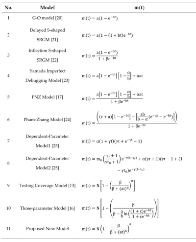
Once the analytical expression for the mean value function m(t) is derived, the model parameters to be estimated in the mean value function can then be obtained with the help of a developed Matlab program based on the least-squares estimate (LSE) method. Five common criteria [18-19], namely the mean squared error (MSE), the sum absolute error (SAE), the predictive ratio risk (PRR), the predictive power (PP), and Akaike’s information criterion (AIC) will be used as criteria for the model estimation of the goodness-of-fit and to compare the proposed model and other existing models as listed in Table 1.
The mean squared error is given by
MSE =∑ ( ( ) ) .
The sum absolute error is given by
SAE = ∑ |m(t ) − y |.
The predictive ratio risk and the predictive power are given as follows: PRR = ∑ ( )( ) , PP = ∑ ( ) .
To compare the all model’s ability in terms of maximizing the likelihood function (MLF) while considering the degrees of freedom, Akaike’s information criterion (AIC) is applied.
AIC = −2 log|MLF| + 2m.
where y is the total number of failures observed at time t ; m is the number of unknown parameters in the model; and m(t ) is the estimated cumulative number of failures at t for i = 1,2, ⋯ , n.
The mean squared error measures the distance of a model estimate from the actual data with the consideration of the number of observations, n, and the number of unknown parameters in the model, m. The sum absolute error is similar to the sum squared error, but the way of measuring the deviation is by the use of absolute values, and sums the absolute value of the deviation between the actual data and the estimated curve. The predictive ratio risk measures the distance of model estimates from the actual data against the model estimate. The predictive power measures the distance of model estimates from the actual data against the actual data. For all five these criteria - MSE, SAE, PRR, PP and AIC - the smaller the value, the closer the model fits relative to other models run on the same data set.
3.2 Estimation of the confidence intervals
In this section, we use Equation (7) to obtain the confidence intervals [18] of the software reliability models in Table 1. The confidence interval is given by
m(t) ± Z / m(t), (7)
where, Z / is 100(1 − α) percentile of the standard normal distribution. Table 1 summarizes the
proposed model and several existing well-known NHPP models with different mean value functions. Note that models 9 and 10 in Table 1 did consider environmental uncertainty.
4. Numerical examples
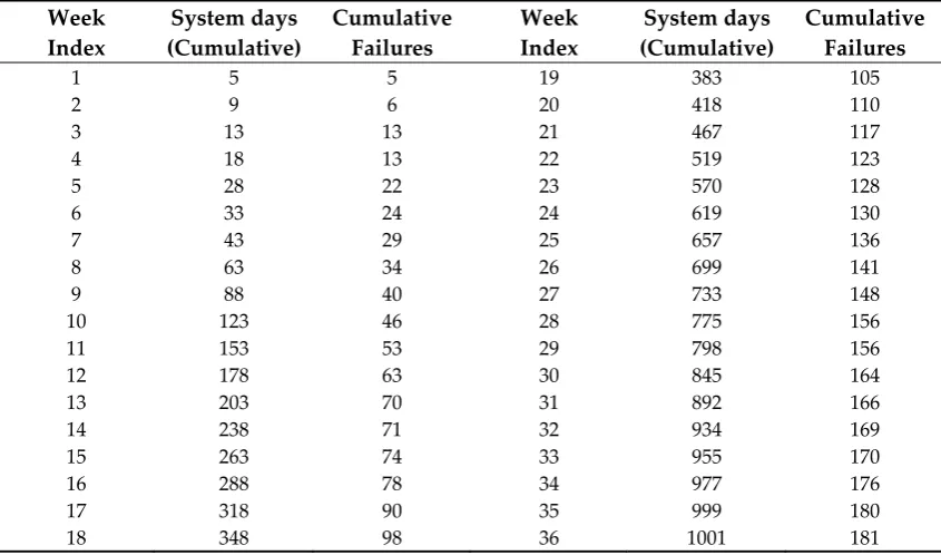
set of failures that were observed during a combination of feature testing and load testing. The test interval that was used in this analysis was a 38 week period between. At times, as many as 11 different BCF frames were being used in parallel to test the software. Thus, to obtain an overall number of days spent testing the software we aggregated the number of days spent testing the software on each frame. The table 3 shows how many days in each week of the test interval that each frame was used for Release 2 testing. The 38 weeks of Release 2 testing accumulates to 1001 days of exposure time.
Table 1. Software reliability models
No. Model ( )
1 G-O model [20] m(t) = a(1 − e )
2
Delayed S-shaped
SRGM [21] m(t) = a(1 − (1 + bt)e )
3 Inflection S-shaped
SRGM [22] m(t) =
a(1 − e )
1 + βe
4
Yamada Imperfect Debugging Model [23]
m(t) = a 1 − e 1 −α
b + αat
5 PNZ Model [17] m(t) =a 1 − e 1 −
α b + αat 1 + βe
6 Pham-Zhang Model [24]
m(t) =
(c + a) 1 − e − b − α (eab − e )
1 + βe
7 Dependent-Parameter Model1 [25]
m(t) = α(1 + γt)(γt + e − 1)
8
Dependent-Parameter Model2 [25]
m(t) = m γt + 1
γt + 1 e ( )+ α(γt + 1)(γt − 1 + (1
− γt )e ( )
9 Testing Coverage Model [13] m(t) = N 1 − β + (at)β
10 Three-parameter Model [16] m(t) = N 1 − β
β −b lna (1 + c)e 1 + ce
11 Proposed New Model m(t) = N 1 − β β + (at)
Table 2. Field failure data for Release 1 – Dataset #1
Month Index System days (Days)
System days
(Cumulative) Failures
Cumulative Failures
1 961 961 7 7
2 4170 5131 3 10
Month Index System days (Days)
System days
(Cumulative) Failures
Cumulative Failures
4 11858 25778 8 32
5 13110 38888 11 43
6 14198 53086 8 51
7 14265 67351 7 58
8 15175 82526 19 77
9 15376 97902 17 94
10 15704 113606 6 100
11 18182 131788 11 111
12 17760 149548 4 115
13 18352 167900 0 115
Table 3. Test data for Release 2 – Dataset #2 Week Index System days (Cumulative) Cumulative Failures Week Index System days (Cumulative) Cumulative Failures
1 5 5 19 383 105
2 9 6 20 418 110
3 13 13 21 467 117
4 18 13 22 519 123
5 28 22 23 570 128
6 33 24 24 619 130
7 43 29 25 657 136
8 63 34 26 699 141
9 88 40 27 733 148
10 123 46 28 775 156 11 153 53 29 798 156 12 178 63 30 845 164 13 203 70 31 892 166 14 238 71 32 934 169 15 263 74 33 955 170 16 288 78 34 977 176 17 318 90 35 999 180 18 348 98 36 1001 181
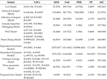
Table 4 and 5 summarize the results of the estimated parameters of all 11 models in Table 1 using the least-squares estimation (LSE) technique and the values of the five common criteria (MSE, SAE, PRR, PP and AIC). We obtained the five common criteria when t = 1,2, ⋯ ,13 from Dataset #1 (Table 2), with exposure time (Cum. System days) from Dataset #2 (Table 3), As can be seen from Table 4, the MSE, SAE, PRR, PP and AIC value for the proposed new model are the lowest values compared to all models. As can be seen from Table 5, the MSE, SAE and PRR value for the proposed new model are the lowest values, and the PP and AIC value for the proposed new model are the second lowest values compared to all models. Table 7 and 8 show confidence intervals of all 11 models from Dataset #1 and #2, respectively (α = 0.05).
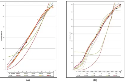
Figure 1 show the graph of the mean value functions for all 11 models for Datasets #1 and #2, respectively. Figure 2 and 3 show that the relative error value of the software reliability model can quickly approach zero in comparison with the other models confirming its ability to provide more accurate prediction. Figure 4 and 5 show the graph of the mean value function and confidence interval each of all 11 models for Datasets #1 and #2, respectively.
Table 4. Model parameter estimation and comparison criteria from Dataset #1
Model LSE's MSE SAE PRR PP AIC
Delayed S-shaped
SRGM a=168.009, b=0.195 20.7414 43.2510 2.3107 0.4295 92.2587 Inflection S-shaped
SRGM
a=134.540, b=0.336,
β=8.939 15.3196 37.2090 0.2120 0.1587 85.3000 Yamada Imperfect
Debugging Model
a=1.130, b=1.110,
α=9.129 33.3890 51.0913 0.3027 0.2495 100.7378 PNZ Model aα=134.549, b=0.3359,
=0.0, β=8.940 17.0223 37.2442 0.2124 0.1588 87.3098
Pham-Zhang Model
a=51.455, b=0.336,
α=289998.1, β=8.939,
c=83.085
19.1495 37.2091 0.2120 0.1587 89.3019
Dependent-Parameter
Model1 α=0.0088, γ=9.996 370.8651 207.3750 60.5062 2.6446 164.5728 Dependent-Parameter
Model2
α=672.637, γ=0.04
t =0.027, m =23.541 215.7784 133.2294 1.1037 8.6260 168.846 Testing Coverage
Model
a=0.242, b=1.701, α=17.967,
β=73.604, N=149.410 25.9244 41.8087 1.4473 0.3601 95.5655 Three-parameter
Model
a=2.980, b=0.336, β=0.080,
c=1105.772, N=135.142 19.1517 37.2107 0.2119 0.1588 89.3053
Proposed New Model
a=0.095, b=15.606,
α=0.085, β=1.855,
N=116.551
11.2281 26.5568 0.2042 0.1558 79.3459
Table 5. Model parameter estimation and comparison criteria from Dataset #2
Model LSE's MSE SAE PRR PP AIC
G-O Model a=291.768, b=0.001 95.3796 299.7160 24.7924 3.4879 198.5419 Delayed S-shaped
SRGM a=168.568, b=0.0057 178.4899 387.7724 7368.5885 7.4923 317.8791 Inflection S-shaped
SRGM
a=200.110, b=0.002,
β=0.059 43.2888 182.9709 10.4336 2.1725 202.0752 Yamada Imperfect
Debugging Model
a=81.999, b=0.0063,
α=0.0014 18.9651 119.1208 3.1804 1.0871 187.7564 PNZ Model aα=67.132, b=0.009,
=0.0019, β=0.0001 18.2406 119.7722 1.5566 0.6869 188.9438
Pham-Zhang Model
a=200.057, b=0.002,
α=9999.433, β=0.058,
c=0.001
46.0819 183.0449 10.4090 2.1698 206.0887
Dependent-Parameter
Model1 α=0.0003, γ=0.866 2075.6677 1411.8412 1165906.4021 17.1338 554.6335 Dependent-Parameter
Model2
α=9.035, γ=0.005
t =48.975, m =49.004 1379.2331 1134.6843 13.0318 156.8519 572.8343 Testing Coverage
Model
a=0.002, b=0.646, α=0.137,
β=8.920, N=7973.501 16.5529 116.0937 0.3033 0.4499 187.4100 Three-parameter
Model
a=0.011, b=0.707, β=8.029,
c=0.000001, N=300.684 34.5762 154.1593 7.7768 1.8500 199.3282
Proposed New Model
a=0.004, b=1.471,
α=0.430, β=78.738,
N=504.403
(a) (b)
Figure 1. Mean value function of all 11 models; (a) Dataset #1; (b) Dataset #2.
Figure 2. Relative error value of 11 models in Table 1 for Dataset #1.
Figure 3. Relative error value of 11 models in Table 1 for Dataset #2.
Time index
Model 1 2 3 4 5 6 7 8 9 10 11 12 13
GO LCL 3.40 10.33 17.83 25.64 33.63 41.77 50.00 58.32 66.70 75.14 83.63 92.16 100.73 UCL 15.43 27.34 38.67 49.69 60.53 71.23 81.83 92.34 102.79 113.18 123.53 133.83 144.10 DS
LCL -0.48 3.73 10.97 20.02 30.02 40.34 50.55 60.36 69.59 78.14 85.96 93.03 99.38 UCL 6.09 16.06 28.34 41.82 55.68 69.37 82.52 94.90 106.36 116.85 126.35 134.88 142.49 IS
LCL 0.73 5.09 11.27 19.14 28.50 38.94 49.88 60.67 70.72 79.59 87.07 93.13 97.91 UCL 9.66 18.57 28.82 40.56 53.62 67.54 81.67 95.29 107.74 118.61 127.68 135.00 140.72 YID
LCL 0.53 6.19 13.66 21.90 30.53 39.37 48.36 57.46 66.64 75.89 85.20 94.55 103.95 UCL 9.16 20.52 32.49 44.49 56.37 68.11 79.74 91.27 102.71 114.10 125.42 136.70 147.94 PNZ
LCL 0.73 5.09 11.26 19.13 28.49 38.92 49.86 60.65 70.69 79.57 87.05 93.12 97.90 UCL 9.66 18.56 28.81 40.55 53.60 67.51 81.64 95.26 107.72 118.58 127.66 134.98 140.71 PZ
LCL 0.73 5.09 11.27 19.14 28.50 38.94 49.88 60.67 70.72 79.59 87.07 93.13 97.91 UCL 9.66 18.57 28.82 40.56 53.62 67.54 81.67 95.29 107.74 118.61 127.68 135.00 140.72 DP1
LCL -0.96 -0.16 2.39 6.71 12.79 20.62 30.21 41.56 54.67 69.54 86.17 104.56 124.70 UCL 2.70 7.18 13.42 21.41 31.16 42.67 55.94 70.97 87.75 106.30 126.60 148.66 172.48 DP2
LCL 14.46 15.79 18.12 21.53 26.13 32.00 39.24 47.92 58.11 69.89 83.32 98.44 115.31 UCL 33.69 35.68 39.08 43.96 50.37 58.34 67.93 79.16 92.08 106.73 123.14 141.36 161.41 TC
LCL -0.29 3.96 10.96 19.79 29.70 40.09 50.49 60.53 69.93 78.53 86.23 93.01 98.87 UCL 6.75 16.49 28.34 41.49 55.25 69.05 82.45 95.10 106.77 117.32 126.68 134.85 141.87 3PDF
LCL 0.73 5.09 11.27 19.15 28.50 38.94 49.88 60.67 70.72 79.59 87.07 93.13 97.91 UCL 9.67 18.57 28.82 40.56 53.62 67.54 81.67 95.29 107.74 118.61 127.68 135.00 140.73 NEW
LCL 0.69 5.37 11.96 19.79 28.61 38.27 48.64 59.62 70.95 81.69 89.62 93.47 94.79 UCL 9.57 19.07 29.88 41.49 53.77 66.66 80.09 93.97 108.03 121.17 130.77 135.41 136.99
(a) (b)
(e) (f)
(g) (h)
(i) (j)
(k)
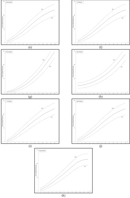
Figure 4. Confidence intervals of all 11 models Dataset #1: (a) GO model; (b) Delayed S-shaped SRGM; (c) Inflection S-shaped SRGM; (d) Yamada Imperfect Debugging Model; (e) PNZ Model; (f) Pham-Zhang Model; (g) Dependent-Parameter Model1; (h) Dependent-Parameter Model2; (i) Testing Coverage Model; (j) Three-parameter Model (k) Proposed New Model.
Time index
Model 5 9 13 18 28 33 43 63 88 123 153 178
GO
LCL -0.91 -0.55 -0.04 0.73 2.49 3.44 5.41 9.54 14.86 22.38 28.78 34.06 UCL 3.82 5.78 7.57 9.68 13.62 15.50 19.15 26.09 34.30 45.16 54.00 61.09 DS
LCL -0.44 -0.69 -0.86 -0.96 -0.79 -0.55 0.24 2.84 7.62 16.27 24.77 32.23 UCL 0.58 1.12 1.74 2.61 4.66 5.81 8.37 14.33 22.95 36.38 48.50 58.66 IS LCL -0.81 -0.23 0.54 1.62 4.03 5.29 7.89 13.22 19.90 29.06 36.62 42.69 UCL 4.57 6.97 9.18 11.77 16.62 18.93 23.40 31.82 41.64 54.37 64.49 72.43 YID
LCL -0.58 0.37 1.51 3.06 6.32 7.98 11.29 17.73 25.28 34.86 42.22 47.82 UCL 5.68 8.73 11.51 14.75 20.74 23.54 28.85 38.52 49.21 62.16 71.82 79.04 PNZ
LCL -0.41 0.77 2.14 3.95 7.68 9.54 13.19 20.05 27.77 37.12 44.04 49.19 UCL 6.34 9.77 12.87 16.48 23.05 26.09 31.77 41.86 52.62 65.16 74.18 80.79 PZ
LCL -0.81 -0.23 0.54 1.63 4.03 5.30 7.90 13.23 19.91 29.07 36.64 42.71 UCL 4.57 6.98 9.18 11.77 16.63 18.94 23.41 31.84 41.66 54.40 64.52 72.46 DP1
LCL -0.14 -0.24 -0.34 -0.46 -0.65 -0.72 -0.85 -0.96 -0.84 -0.21 0.77 1.90 UCL 0.15 0.28 0.42 0.60 1.00 1.21 1.68 2.74 4.33 7.02 9.76 12.36 DP2
LCL 36.10 36.08 36.04 35.98 35.81 35.70 35.45 34.84 33.93 32.62 31.61 30.93 UCL 63.81 63.78 63.73 63.65 63.42 63.28 62.95 62.13 60.93 59.18 57.82 56.90 TC
LCL 1.34 3.18 4.87 6.81 10.33 11.96 15.02 20.58 26.81 34.64 40.78 45.58 UCL 11.12 15.01 18.17 21.58 27.35 29.89 34.53 42.62 51.31 61.87 69.94 76.16 3PDF
LCL -0.76 -0.09 0.77 1.96 4.58 5.94 8.71 14.31 21.20 30.46 37.96 43.90 UCL 4.85 7.41 9.76 12.51 17.64 20.07 24.74 33.47 43.50 56.27 66.25 74.00 NEW
LCL 1.50 3.41 5.13 7.12 10.70 12.36 15.47 21.12 27.45 35.43 41.69 46.60 UCL 11.49 15.44 18.65 22.10 27.93 30.50 35.20 43.38 52.19 62.92 71.13 77.48 Time index
Model 208 238 263 288 318 348 383 418 467 519 570 619
GO LCL 40.28 46.39 51.37 56.26 62.00 67.60 73.95 80.11 88.41 96.83 104.70 111.91 UCL 69.30 77.20 83.57 89.76 96.95 103.90 111.72 119.25 129.31 139.43 148.83 157.40 DS
LCL 41.33 50.31 57.57 64.55 72.46 79.84 87.72 94.83 103.52 111.25 117.51 122.47 UCL 70.66 82.22 91.40 100.11 109.89 118.92 128.48 137.04 147.43 156.62 164.02 169.86 IS
LCL 49.68 56.35 61.66 66.76 72.59 78.12 84.22 89.94 97.36 104.54 110.94 116.53 UCL 81.42 89.87 96.53 102.86 110.05 116.82 124.24 131.15 140.07 148.65 156.24 162.86 YID
LCL 54.00 59.68 64.08 68.22 72.91 77.34 82.24 86.89 93.09 99.38 105.33 110.90 UCL 86.90 94.04 99.53 104.67 110.45 115.87 121.83 127.47 134.95 142.49 149.58 156.20 PNZ
LCL 54.79 59.89 63.84 67.58 71.85 75.93 80.51 84.96 91.02 97.31 103.41 109.22 UCL 87.90 94.31 99.24 103.88 109.14 114.14 119.74 125.13 132.45 140.01 147.29 154.21 PZ LCL 49.70 56.37 61.69 66.78 72.61 78.14 84.24 89.96 97.38 104.55 110.94 116.53
UCL 81.45 89.90 96.55 102.88 110.07 116.85 124.26 131.17 140.09 148.66 156.25 162.86 DP1
LCL 3.62 5.75 7.83 10.19 13.40 17.02 21.74 27.02 35.34 45.34 56.34 68.01 UCL 15.85 19.74 23.29 27.13 32.10 37.48 44.26 51.60 62.80 75.86 89.86 104.40 DP2
LCL 30.39 30.21 30.37 30.84 31.83 33.30 35.66 38.71 44.19 51.52 60.24 70.02 UCL 56.17 55.93 56.15 56.78 58.11 60.09 63.22 67.25 74.37 83.76 94.75 106.88 TC LCL 51.03 56.22 60.36 64.36 69.00 73.47 78.51 83.38 89.93 96.59 102.88 108.70 UCL 83.14 89.70 94.90 99.89 105.63 111.13 117.30 123.22 131.14 139.15 146.66 153.59 3PDF
LCL 50.68 57.08 62.15 67.00 72.52 77.76 83.54 88.98 96.09 103.04 109.34 114.96 UCL 82.69 90.79 97.14 103.15 109.97 116.39 123.42 130.00 138.55 146.86 154.35 161.00 NEW
LCL 52.20 57.52 61.77 65.88 70.65 75.26 80.44 85.45 92.20 99.05 105.50 111.48 UCL 84.62 91.33 96.66 101.77 107.66 113.32 119.65 125.73 133.87 142.10 149.79 156.88 Time index
GO
LCL 117.28 122.99 127.45 132.76 135.58 141.15 146.47 151.03 153.23 155.50 157.72 157.91 UCL 163.75 170.48 175.71 181.93 185.23 191.72 197.91 203.19 205.75 208.37 210.93 211.17 DS
LCL 125.68 128.70 130.77 132.95 133.98 135.79 137.25 138.32 138.78 139.22 139.61 139.65 UCL 173.64 177.17 179.61 182.15 183.36 185.47 187.18 188.42 188.96 189.47 189.93 189.97 IS
LCL 120.52 124.62 127.70 131.23 133.05 136.53 139.70 142.30 143.52 144.75 145.93 146.03 UCL 167.57 172.38 176.00 180.14 182.27 186.33 190.03 193.06 194.48 195.91 197.28 197.40 YID
LCL 115.14 119.78 123.51 128.08 130.57 135.64 140.70 145.20 147.46 149.81 152.17 152.38 UCL 161.22 166.70 171.08 176.45 179.37 185.30 191.19 196.44 199.05 201.79 204.52 204.77 PNZ
LCL 113.71 118.66 122.67 127.62 130.33 135.87 141.41 146.37 148.85 151.45 154.05 154.29 UCL 159.53 165.38 170.10 175.91 179.08 185.56 192.02 197.79 200.67 203.69 206.70 206.97 PZ
LCL 120.52 124.61 127.69 131.22 133.04 136.51 139.68 142.28 143.50 144.73 145.91 146.01 UCL 167.57 172.38 175.99 180.13 182.26 186.32 190.01 193.04 194.46 195.89 197.25 197.37 DP1
LCL 77.80 89.38 99.33 112.35 119.81 135.80 152.79 168.81 177.12 186.03 195.17 196.01 UCL 116.43 130.48 142.43 157.92 166.73 185.49 205.24 223.73 233.27 243.48 253.91 254.86 DP2 LCL 78.53 88.88 97.96 110.03 117.04 132.22 148.53 164.05 172.14 180.85 189.79 190.62 UCL 117.33 129.87 140.79 155.17 163.46 181.29 200.29 218.24 227.55 237.54 247.77 248.72 TC
LCL 113.09 117.82 121.56 126.08 128.52 133.40 138.17 142.33 144.39 146.52 148.63 148.82 UCL 158.79 164.38 168.79 174.11 176.96 182.68 188.24 193.10 195.49 197.96 200.41 200.63 3PDF
LCL 119.05 123.32 126.60 130.46 132.48 136.43 140.16 143.32 144.84 146.39 147.91 148.04 UCL 165.83 170.86 174.72 179.24 181.60 186.22 190.57 194.25 196.01 197.82 199.58 199.73 NEW
LCL 115.97 120.80 124.61 129.21 131.68 136.62 141.43 145.62 147.68 149.81 151.92 152.11 UCL 162.20 167.89 172.38 177.78 180.67 186.44 192.05 196.92 199.31 201.79 204.23 204.45
(a) (b)
(e) (f)
(g) (h)
(i) (j)
(k)
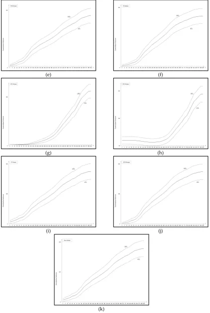
Figure 5. Confidence intervals of all 11 models Dataset #2: (a) GO model; (b) Delayed S-shaped SRGM; (c) Inflection S-shaped SRGM; (d) Yamada Imperfect Debugging Model; (e) PNZ Model; (f) Pham-Zhang Model; (g) Dependent-Parameter Model1; (h) Dependent-Parameter Model2; (i) Testing Coverage Model; (j) Three-parameter Model (k) Proposed New Model.
Generally, existing models are applied to software testing data and then used to make predictions on the software failures and reliability in the field. Here, the important point is that the test environment and operational environment are different from each other. In this paper, we discussed a new software reliability model based on a Weibull fault detection rate function subject to the uncertainty of operating environments. Table 4 and 5 summarized the results of the estimated parameters of all 11 models in Table 1 using the LSE technique and the five common criteria (MSE, SAE, PRR, PP and AIC) value for two data sets. As can be seen from Table 4, the MSE, SAE, PRR, PP and AIC value for the proposed new model are the lowest values compared to all models. As can be seen from Table 5, the MSE, SAE and PRR value for the proposed new model are the lowest values compared to all models. Finally, we show confidence intervals of all 11 models from Dataset #1 and #2, respectively, in Table 7 and 8. By estimating the confidence interval, we will help to find the optimal software reliability model at different confidence levels.
Acknowledgement: This research was supported by Basic Science Research Program through the National Research Foundation of Korea (NRF) funded by the Ministry of Education (NRF-2015R1D1A1A01060050). Author Contributions: The three authors equally contributed to the paper.
Conflicts of Interest: The authors declare no conflict of interest.
References
1. Fang, C. C.; Yeh, C. W. Confidence interval estimation of software reliability growth models derived from stochastic differential equations. Industrial Engineering and Engineering Management (IEEM), IEEE International Conference on. IEEE, 2011, 1843-1847.
2. Yamada, S.; Osaki, S. Software reliability growth modeling: models and applications. IEEE Trans. Softw. Eng. 1985, 11(12), 1431–1437.
3. Yin, L.; Trivedi, K.S. Confidence interval estimation of NHPP-based software reliability models. Proceedings of the 10th International Symposium on Software Reliability Engineering, November, 1999, 6-11.
4. Huang, C. Y. Performance analysis of software reliability growth models with testing effort and change-point, J. Syst. Softw, 2005, 76, 181-194.
5. Chatterjee, S.; Singh, J. B. A NHPP based software reliability model and optimal release policy with logistic-exponential test coverage under imperfect debugging. Int. J. Syst. Assur. Eng. Manag. 2014, 5(3), 399-406.
6. Chatterjee, S.; Shulka, A. Software reliability modeling with different type of faults incorporating both imperfect debugging and change point. Proceedings of 4th International Conference on Reliability, Infocom, Technologies and Optimization, September, 2015, 1-5.
7. Yang, B.,; Xie, M. A study of operational and testing reliability in software reliability analysis. Reliab. Eng. Syst. Saf. 2000, 70, 323-329.
8. Huang, C. Y.; Kuo, S. Y.; Lyu, M. R.; Lo, J. H. Quantitative software reliability modeling from testing from testing to operation. Proceedings of the International Symposium on Software Reliability Engineering, IEEE, Los Alamitos, CA, USA, 2000, 72-82.
9. Zhang, X.; Jeske, D.; Pham, H. Calibrating software reliability models when the test environment does not match the user environment. Appl. Stoch. Models. Bus. Ind. 2002, 18, 87-99.
10. Teng, X.; Pham, H. A new methodology for predicting software reliability in the random field environments. IEEE Trans. Reliab. 2006, 55(3), 458-468.
11. Pham, H. A software reliability model with Vtub-Shaped fault-detection rate subject to operating environments. Proceeding of the 19th ISSAT International Conference on Reliability and Quality in Design, August 5-7, Hawaii, USA, 2013, 33-37.
12. Pham, H. A new software reliability model with Vtub-Shaped fault detection rate and the uncertainty of operating environments. Optimization. 2014, 63(10), 1481-1490.
14. Honda, K.; Nakai, H.; Washizaki, H.; Fukazawa, Y. Predicting time range of development based on generalized software reliability model. Proceedings of 21st Asia-Pacific Software Engineering Conference, 2014, 351-358.
15. Pham, H. A generalized fault-detection software reliability model subject to random operating environments. Vietnam J. Comp. Sci. 2016, 3, 145-150.
16. Song, K. Y.; Chang, I. H.; Pham, H. A Three-parameter fault-detection software reliability model with the uncertainty of operating environments, J. Syst. Sci. Syst. Eng. 2017, 26(1), 121-132.
17. Pham, H.; Nordmann, L.; Zhang, X. A general imperfect software debugging model with S-shaped fault detection rate. IEEE Trans. Reliab. 1999, 48(2), 169–175.
18. Pham, H. System Software Reliability, Springer, London, 2006.
19. Akaike, H. A new look at statistical model identification. IEEE Trans. Autom. Control. 1974, 19, 716-719. 20. Goel, A. L.; Okumoto, K. Time dependent error detection rate model for software reliability and other
performance measures. IEEE Trans. Reliab. 1979, 28(3), 206–211.
21. Yamada, S.; Ohba, M.; Osaki, S. S-shaped reliability growth modeling for software fault detection. IEEE Trans. Reliab. 1983, 32(5), 475–484.
22. Ohba, M. Inflexion S-shaped software reliability growth models. Stochastic Models in Reliability Theory. Osaki, S., & Hatoyama, Y. (eds.). Springer-Verlag, Berlin, 1984, 144–162.
23. Yamada, S.; Tokuno, K.; Osaki, S. Imperfect debugging models with fault introduction rate for software reliability assessment. Int. J.Syst. Sci. 1992, 23(12), 2241–2252.
24. Pham, H.; Zhang, X. An NHPP software reliability models and its comparison. Int. J. Reliab. Qual. Saf. Eng. 1997, 4(3), 269–282.
25. Pham, H. Software Reliability Models with Time Dependent Hazard Function Based on Bayesian Approach. Int. J. Automat. Comput. 2007, 4(4), 325-328.