(will be inserted by the editor)
Improving Resource Location with Locally Precomputed
Partial Random Walks
V´ıctor M. L´opez Mill´an · Vicent Cholvi ·
Luis L´opez · Antonio Fern´andez Anta
the date of receipt and acceptance should be inserted later
Abstract Random walks can be used to search complex networks for a desired resource. To reduce search lengths, we propose a mechanism based on building random walks connecting together partial walks (PW) previously computed at each network node. Resources found in each PW are registered. Searches can then jump over PWs where the resource is not located. However, we assume that perfect recording of resources may be costly, and hence, probabilistic structures like Bloom filters are used. Then, unnecessary hops may come from false positives at the Bloom filters. Two variations of this mechanism have been considered, depending on whether we first choose a PW in the current node and then check it for the resource, or we first check all PWs and then choose one. In addition, PWs can be either simple random walks or self-avoiding random walks. Analytical models are provided to predict expected search lengths and other magnitudes of the resulting four mechanisms. Simulation experiments validate these predictions and allow us to compare these techniques with simple random walk searches, finding very large reductions of expected search lengths.
Keywords Random walks · self-avoiding random walks · network search·
resource location·search length
This research was supported in part by Comunidad de Madrid grant S2009TIC-1692, Spanish MINECO grant TEC2011-29688-C02-01, Spanish MINECO grant TIN2011-28347-C02-01, Bancaixa grant P11B2010-28, and National Natural Science Foundation of China grant 61020106002.
V. M. L´opez Mill´an
Universidad CEU San Pablo, Spain E-mail: [email protected] Vicent Cholvi
Universitat Jaume I, Spain E-mail: [email protected] Luis L´opez
Universidad Rey Juan Carlos, Spain E-mail: [email protected] Antonio Fern´andez Anta
1 Introduction
A random walk in a network is a routing mechanism that chooses the next node to visit at random among the neighbors of the current node. Random walks have been extensively studied in mathematics, and have been used in a wide range of applications such as statistic physics, population dynamics, bioinformatics, etc. When applied to communication networks, random walks have had a profound impact on algorithms and complexity theory. Some of the advantages of random walks are their simplicity, their small processing power consumption at the nodes, and the fact that they need only local information, avoiding the communication overhead necessary in other routing mechanisms. An important application of random walks has been the search for resources held in the nodes of a network, also known as the resource location problem. Roughly speaking, the problem consists of finding a node that holds the re-source, starting at some source node. Random walks can be used to perform such a search as follows. It is checked first if the source node holds the resource. If it does not, the search hops to a random neighbor, that repeats the process. The search proceeds through the network in this way until a node that holds the resource is found. Due to the random nature of the walk, some nodes may be visited more than once (unnecessarily from the search standpoint), while other nodes may remain unvisited for a long time. The number of hops to find the resource is thesearch length of that walk. The performance of this direct application of random walks to network search has been studied in [1–5].
The use of random walks for resource location has several clear applica-tions, like unstructured peer-to-peer (P2P) file sharing systems or content-centric networks (CCN) [6]. The latter are networks in which the key elements are named content chunks, which are requested by users using the content name. Content chunks have to be efficiently located and transferred to be con-sumed by the user. The techniques described in this paper could be used in the context of CCN to locate content chunks.
anal-yses. These assumptions provide generality to our model, since a probability of p= 0 models the case in which the full list of resources found are stored (instead of using a Bloom filter).
We provide an analytical model for the choose-first PW-RW technique, with expressions for theexpected search length, theoptimal length of the par-tial walks, and for the optimal expected search length. We found that, when the probability of false positives in Bloom filters is small, the optimal ex-pected search length is proportional to the square root of the exex-pected search length achieved by simple random walks, in agreement with the results in [8]. Another interesting finding is that the optimal length of the partial walks does not depend on the probability of false positives of the Bloom filters. We also provide analytical models for the choose-first PW-SAW mechanism as well as for the check-first variations, which predict their expected search length. Then, the predictions of the models are validated by simulation experiments in three types of randomly built networks: regular, Erd˝os-R´enyi, and scale-free. These experiments are also used to compare the performance of the four mechanisms, and to investigate the influence of parameters as the false positive probability and the number of partial walks per node. Finally, we have com-pared the performance of the four search mechanisms with respect to simple random walk searches. For choose-first PW-RW we have found a reduction in the average search length ranging from around 98% to 88%. For choose-first PW-SAW such a reduction is even bigger, ranging from 12% to 5% with re-spect to PW-RW. Check-first PW-RW and PW-SAW can achieve still larger reductions increasing the number of PWs available at each node.
Related Work. Das Sarma et al. [8] proposed a distributed algorithm to obtain a random walk of a specified lengthℓin a number of rounds1 proportional to
√
ℓ. First, every node in the network prepares a number of short (random) walks departing from itself. The second phase takes place when a random walk of a given length starting from a given source node is requested. One of the short walks of the source node is randomly chosen to be the first part of the requested random walk. Then, the last node of that short walk is processed. One of its short walks is randomly chosen, and it isconnected to the previous short walk. The process continues until the desired length is reached.
Hieungmany and Shioda [9] proposed a random-walk-based file search for P2P networks. A search is conducted along the concatenation of hop-limited shortest path trees. To find a file, a node first checks itsfile list (i.e., an index of files owned by neighbor nodes). If the requested file is found in the list, the node sends the file request message to the file owner. Otherwise, it randomly selects a leaf node of the hop-limited shortest path tree, and the search follows that path, checking thefile list of each node in it.
The use of partial random walks in resource location has been proposed in [10] for networks with dynamic resoures. Our work in this paper incorporates
1 Around is a unit of discrete time in which every node is allowed to send a message to
efficient storage by means of Bloom filters, in the context of static resources. The use of SAWs as PWs is also proposed and compared with simple RWs.
Structure. The next section presents a model for the four search mechanisms proposed. Choose-first PW-RW is analyzed and evaluated in Section 3. For clarity, choose-first PW-SAW is covered separately in Section 4. Similarly, check-first PW-RW/PW-SAW are presented in Section 5.
2 Model
Let us consider a randomly built network ofN nodes and arbitrary topology, whose nodes hold resources randomly placed in them. Resources are unique, i.e., there is a single instance of each resource in the network. The resource location problem is defined as visiting the node that holds the resource, starting from a certain node (the source node). For each search, the source node is chosen uniformly at random among all nodes in the network.
The search mechanisms proposed in this paper exploit the idea of efficiently buildingtotal random walks frompartial random walks available at each node of the network. This process comprises two stages:
(1) Partial walks construction. Every node i in the network precomputes a set Wi of w random walks in an initial stage before the searches take place.
Each of these partial walks has lengths, starting atiand finishing at a node reached aftershops. In the PW-RW mechanism, the partial walks computed in this stage are simple random walks. During the computation of each partial walk in Wi, node i registers the resources held by the s first nodes in the
partial walk (fromi to the one before the last node). As mentioned, for gen-erality, we assume that the resources found are stored in a Bloom filter. This information will be used in Stage 2. Bloom filters are space-efficient random-ized data structures to store sets, supporting membership queries. Thus, the Bloom filter of a partial walk can be queried for a given resource. If the result is negative, the resource is not in any of the nodes of the partial walk. If the result is positive, the resource is in one of the nodes of the partial walk, un-less the result was afalse positive, which occurs with a certain probabilityp.2 The size of the Bloom filters can be designed for a target (small)pconsidered appropriate. A variation of the partial walk construction mechanism consists of using PWs that areself-avoiding walks (SAW). The resulting mechanism, called PW-SAW, is analyzed in Section 4.
(2) The searches. After the PWs are constructed, searches are performed in the following fashion when the choose-first PW-RW/PW-SAW mechanisms are used. When a search starts at a nodeA, a PW inWA is chosen uniformly
2 More concretely,p is the probability of obtaining a positive result conditioned on the
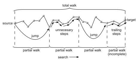
Fig. 1: An example of search, using PWs of lengths= 6.
at random. Its Bloom filter is then queried for the desired resource. If the re-sult is negative, the searchjumpsto nodeB, the last node of that partial walk. The process is then repeated at B, so that the search keeps jumping in this way while the results of the queries are negative. When at a nodeC, the query to the Bloom filter (of the PW randomly chosen from WC) gives a positive
result, the searchtraverses that partial walk looking for the resource until the resource is found or the partial walk is finished. If the resource is found, the search stops. If the search reaches the last nodeDof the partial walk without having found the resource in the previous nodes, it means that the result of the Bloom filter query was a false positive. The search then randomly chooses a partial walk in WD and decides whether to jump over it or to traverse it
depending on the result of the query to its Bloom filter. A variation consists of first checking all PWs of the node for the desired resource, and then randomly choosing among the ones with a positive result. The resulting mechanisms, called check-first PW-RW/PW-SAW are analyzed in Section 5.
In this work, we are interested in the number of hops to find a resource (when PWs of length s are used), which is defined as thesearch length and denoted Ls. Some of these hops are jumps (over PWs) and other are steps
(traversing PWs). In turn, we distinguish betweentrailing steps, taken when the resource is found, andunnecessary steps, taken when the resource is not found. The search length is a random variable that takes different values when independent searches are performed. Thesearch length distribution is defined as the probability distribution of the search length random variable. We are in-terested in finding theexpected search length, denotedLs. Figure 1 summarizes
the behavior of the search mechanisms.
3 Choose-First PW-RW
3.1 Analysis of Choose-First PW-RW
We make an additional assumption in order to simplify this analysis. Once a PW has been used in the total walk of a search, it is never reused again in that total walk or in any other searches. Thus we guarantee that the total walks are true random walks. This implies that in practice each node needs to have a large number of precomputed partial walks (w), assumption that would compromise the benefits of the proposed mechanism in practice. Simulations in Section 3.2 show that real cases with smallwbehave very similarly to the base case provided by this analysis.
Let Ls be the random variable representing the number of hops in the
search (i.e., its length) when PWs of length sare used. The expected search length is denoted byLs. LetLbe the random variable representing the number
of hops of the corresponding total walk. Its expected search length is denoted
L. Making use of the assumption that partial walks are never reused, L can be viewed as the length of a search based on a simple random walk in the considered network, andL as the expected search length of random walks in that network. Then, we can state the following theorem:
Theorem 1 If the expected number of trailing steps is assumed to be uniformly distributed in[0, s−1]3, then the expected search length is:
Ls=
µ
s
2 + 2L+ 1
2s −1
·(1−p) +L·p. (1)
Proof LetP,J,U andT be random variables representing the number of par-tial walks, jumps, unnecessary steps and trailing steps in a search, respectively. Their expectations are denoted asP,J,U andT. Since hops in a search can be jumps, unnecessary steps or trailing steps, it follows that,Ls=J+U+T.
Then, the expected search length for partial walks of sizesis4L
s=J+U+T .
The expected number of jumps can be obtained from the expected number of partial walks in the search (P) and from the probability of false positive (p) as J =P·(1−p),sinceJ follows a binomial distribution B(P,1−p), where the number of experiments is the random variable representing the number of partial walks in a search (P) and the success probability is the probability of obtaining a negative result in a Bloom filter query (1−p).5
3 This is, in fact, a pessimistic assumption. The distribution of trailing steps is
approxi-mately uniform, but shorter walks have a slightly higher probability than longer ones. This can be shown analytically and has been confirmed in our experiments (see Appendix A). Therefore, the expected value in our analysis, derived from a perfectly uniform distribution, is slightly higher than the real average value.
4 In the following, we make implicit use of the linearity properties of expectations of
random variables.
5 If Y is a random variable with a binomial distribution with success probabilityp, in
For the expected number of unnecessary steps, U =P·p·s,sinceP·pis the expected number of false positives in the search and each contributes with
sunnecesary steps. The number of partial walks in a search can be obtained dividing the length of the total walk by the size of a PW: P =¥L
s
¦
= L−T
s .
Then, the expected number of partial walks in a search isP =L−T
s .
Since we assume that the expected number of trailing steps is uniformly distributed between 0 and (s−1), its expectation isT =s−1
2 .Then we have:
Ls=
µ
s
2+ 2L+ 1
2s −1
+p·
µ
L−
µ
s
2+ 2L+ 1
2s −1
¶¶
,
where the first term is the expectation of the search length for a “perfect” Bloom filter (one that never returns a false positive when the resource is not in the filter, i.e.,p= 0), and the second term is the expectation of the additional search length due to false positives (p6= 0).
Reorganizing to make explicit the contributions of a perfect filter and of a “broken” filter (one that always returns a false positive result when the resource is not in the filter, i.e.,p= 1), we have that:
Ls=
µs
2 + 2L+ 1
2s −1
·(1−p) +L·p.
From this theorem and using calculus, we have the following corollary.
Corollary 1 The optimal length of the partial walks, i.e., the length of the partial walks that minimizes the expected search length, is:
sopt=
p
2L+ 1.
The obtained value needs to be rounded to an integer, which is omitted in the notation. Observe thatthe optimal length of the partial walks is independent from the probability of false positives in the Bloom filters, while the expected search length (Ls) does of course depend on it.
Corollary 2 The optimal expected search length, i.e., the expected search length when partial walks of optimal length are used, is:
Lopt=
³p
2L+ 1−1´(1−p) +L p= (sopt−1) (1−p) +L p. (2)
This result is an interesting relation between the optimal length of the search and the optimal length of the PWs. If we consider perfect Bloom filters (p= 0), we have Lopt=sopt−1,which for large L (e.g. for large networks) becomes
Lopt≈sopt. Therefore, we have found that, for largeN andp= 0,the optimal
expected search length approximately equals the optimal length of the partial walks. For arbitrary values ofp, the equation above shows thatLopt is linear
inp.
Cost of Precomputing PWs. Since searches use the partial walks precomputed by the nodes, the cost of this computation must be taken into account. We mea-sure this cost as the number of messagesCp that need to be sent to compute
all the PWs in the network. This quantity has been chosen to be consistent with our measure of the performance of the searches. Indeed, eachhop taken by a search can be alternatively considered as a message sent. In addition,
Cp is independent from other factors like the processing power of nodes, the
bandwidth of links and the load of the network. The cost of precomputing a set of PWs can be simply obtained as Cp =N w(s+ 1), since each of theN
nodes in the network computesw partial walks, sending smessages to build each of them plus one extra message to get back to its source node.
Let’s suppose that each node starts on the average b searches that are processed by the network with the set of PWs precomputed initially. We define
Cs to be the total number of messages needed to complete those searches. If
the expected number of messages of a search isLs+ 1 (counting the message
to get back to the source node), we have thatCs=N b(Ls+ 1). Now, defining
Ctas theaverage total cost per search, we can write:
Ct=
Cs+Cp
N b = (Ls+ 1) + w
b(s+ 1).
The second term in this equation is the contribution to the cost of the precomputation of the PWs. This contribution will remain small provided that the number of searches per node in the interval is large enough.
3.2 Performance Evaluation
The goal of this section is to apply the model for choose-first PW-RW presented in the previous section to real networks, and to validate its predictions with data obtained from simulations. Three types of networks have been chosen for the experiments: regular networks (constant node degree), Erd˝os-R´enyi (ER) networks and scale-free networks (with power law on the node degree). A network of each type and sizeN = 104 has been randomly built with the method proposed by Newman et al. [11] for networks with arbitrary degree distribution, setting their average node degree to k = 10. Each network is constructed in three steps: (1) a preliminary network is constructed according to its type; (2) its degree distribution is extracted, and (3) the final (random) network is obtained feeding the Newman method with that degree distribution. For each experiment, 106 searches have been performed, with the source node chosen uniformly at random among the N nodes. Likewise, the resource has been placed in a node chosen uniformly at random for each experiment.
0 500 1000 1500 2000 2500 3000 3500
0 50 100 150 200 250 300 350 400
expected search length (hops)
partial walks size (hops) 100
150 200 250 300 350
0 50 100 150 200 250 300 350 400
sopt
E(L)opt
scale-free, p=0 (simul) (model) ER, p=0 (simul) (model) regular, p=0 (simul) (model)
(a)
0 2000 4000 6000 8000 10000 12000 14000 16000 18000
0 0.2 0.4 0.6 0.8 1
optimal expected search length (hops)
probability of false positives
E(L) regular
ER scale-free
(b)
Fig. 2: (a) Expected search length (Ls) vs.swhenp= 0 in the three networks.
(b) Optimal expected search length (Lopt) vs.p.
expected search length as a function of the size of the PWs.6 Figure 2(a) provides plots of the expected search lengths (Ls) given by Equation 1 as a
function of the size of the PWs (s), when the probability of a false positive in the Bloom filter is set top= 0, for the three types of networks considered. Results from the analytical model are shown as curves while simulation data are shown as points. The curves for the three networks show a minimum point (sopt, Lopt). This behavior is due to the fact that, whensis small, the number
of jumps needed to reach a PW containing the chosen resource grows, therefore increasing the value ofL. In turn, for larger values ofs, the number of trailing steps within the last PW grows, also increasing the value ofL.
Figure 2(b) illustrates (using Equation 2 and taking into account the fact that sopt is independent from the value of p) the optimal expected search
length (Lopt) as a function of the probability of false positives (p). It can be
seen that it grows linearly: the regular network exhibits the smallest slope, followed by the ER network and then by the scale-free network. For p = 1, Equation 2 degenerates toLopt=L, since the search performs all the hops of
the total walk (i.e., it is a random walk). In fact, Equation 1 also degenerates to Ls = L in this case, meaning that the expected search length is that of
random walk searches regardless the size of the PWs (s).
Distributions of Search Lengths in Choose-First PW-RW. The aim of this section is to experimentally explore how the use of PWs affects the statisti-cal distribution of search lengths. We first obtain the lengths distributions of searches using PWs that are never reused. Later in this section we will discuss
6 For each network, the expected length of a random walk search (L) is needed. We
esti-mate these expected values by simulating 106 simple random walk searches and averaging
their lengths in each of the networks (these average search lengths are denoted using low-ercase (l) to distinguish them from the actual expected value (L) in the model. The values obtained from the experiments are:lreg = 11246,lER= 12338, and lsf = 15166). These
0 1000 2000 3000 4000 5000 6000
0 200 400 600 800 1000 1200
number of searches
search length s = 150 average: 148.8
s = 1000 average: 502.6 s = 50
average: 248.9
frequency for s=50 average frequency for s=150 average frequency for s=1000 average
(a) Search lengths forp= 0 and severals.
0 1000 2000 3000 4000 5000 6000
0 200 400 600 800 1000 1200 1400
number of searches
search length p = 0 average: 148.8
p = 0.01 average: 259.9
p = 0.1 average: 1259.7 frequency for p=0
average frequency for p=0.01 average frequency for p=0.1 average
(b) Search lengths for sopt and for p =
0,0.01,0.1.
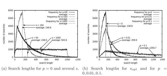
Fig. 3: Distributions of search lengths for non-reused PWs (regular network)).
the effect of having a limited number of partial random walks that are reused. We consider each random walk to be the total walk of a search based on PWs. For each original random walk, we break it in pieces of sizes, which are taken as the PWs that make up the total walk. Then we consider a search that uses those PWs and count the number of hops (jumps plus trailing steps plus un-necessary steps). This gives the length of the search if it had been constructed using those (precomputed) PWs. Note that the PWs are not reused because they are obtained from independent (real) random walks.
The search length distributions in the regular network for p = 0 and for several values ofs are shown in Figure 3(a). The plots also show, as vertical bars, the average search lengths computed from each distribution. These av-erage values are very close to the expected values calculated with Equation 1 (L50 = 248.9, L150 = 149.0 and L1000 = 510.2). Therefore, our model accu-rately predicts average lengths of searches based on PWs of sizesin the three types of networks considered in our experiments.
As for the shape of the distributions, we observe that for low s(s= 50 in Figure 3(a)) the search lengths are dominated by the number of jumps, which is proportional to the length of the total walk. On the other hand, for high
s (s= 1000 in Figure 3(a)) the distribution adopts a rather uniform shape. Search lengths are dominated here by the number of trailing steps in the last PW, and this has approximately an uniform distribution between 0 and
s−1, as mentioned earlier. The optimal length for the PWs,sopt(s= 150 in
Figure 3(a)), represents a transition point between these two effects. The shape is such that the values around the average search length (which approximately equalssopt, according to Equation 2) are also the most frequent.
Once it has been found the optimal length for the PWs sopt (which is
known to be independent of the value of p), we investigate the effect of the
provided in [5]), which produces the following results: lreg = 11095, lER = 12191, and
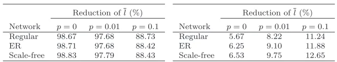
Table 1: Reductions of average search lengths.
(a) PW-RW with respect to RW searches Reduction ofl(%) Network p= 0 p= 0.01 p= 0.1 Regular 98.67 97.68 88.73 ER 98.71 97.68 88.42 Scale-free 98.83 97.79 88.43
(b) PW-SAW with respect to PW-RW Reduction ofl(%) Network p= 0 p= 0.01 p= 0.1 Regular 5.67 8.22 11.24
ER 6.25 9.10 11.88
Scale-free 6.53 9.75 12.65
probability of false positive of Bloom filters in these distributions. Figure 3(b) shows the distributions of search lengths (histograms) for the regular network whens=soptand for several values ofp. It can be seen that the distributions
get wider and lower as p grows, pushing average search lengths to higher values, in accordance with Figure 2(b). However, we observe that the most frequent lengths remain the same regardless of the value ofp. For p= 0, the most frequent value for each network approximately equals the average search length which, in turn, approximately equals the optimal length of the PWs (sopt= 150 for the regular network). For greater values ofp, the average search
length grows while the most frequent value stays the same.
Regarding the distributions for the ER and the scale-free networks, they have similar shapes and are not shown here. However, we have used these distributions to obtain Table 1(a) (explained below).
Effect of reusing PWs. At this point, we note that we have been assuming that PWs are never reused. However, in practical scenarios it seems quite reasonable to consider a limited number of partial random walks that are reused. In Appendix C we have explored the distributions of search lengths when the total walks are built reusing a limited numberwof PWs precomputed in each node. As it can be readily seen there, we conclude that, for the types of networks in our experiment, just two precomputed PWs per node are enough to obtain searches whose lengths are statistically similar to those that would be obtained with PWs that are not reused. So, we can say that our results for not reused PWs are also valid when reusing a limited number of PWs.
4 Choose-First PW-SAW
As it was pointed in Section 2 when we introduced the PW construction mech-anism in Stage 1, a possible variation consists of using self-avoiding walks (SAW) instead of simple random walks. The resulting search mechanism is called PW-SAW. The basic idea is to revisit less nodes, thus increasing the chances of locating the desired resource. In short, a SAW chooses the next node to visit uniformly at random among the neighbors that have not been visited so far by the walk. If all neighbors have already been visited, it chooses uniformly at random among all neighbors, like a simple random walk.
Analysis of Choose-First PW-SAW. When PWs are self-avoiding walks, their concatenation is not a random walk, and hence Theorem 1 is no longer valid. We state a new theorem for the choose-first PW-SAW mechanism, proving it using a different approach.
Theorem 2 If the expected number of trailing steps is assumed to be uniformly distributed in[0, s−1], then the expected search length of PW-SAW is
Ls=
1
N
X
k
nk
µ
1
ptp(k)·
(pn(k) +s·pf p(k)) +
s−1
2
.
The probabilities that the query of the Bloom filter of the chosen PW in the current node returns a (true) negative, a true positive, and a false positive result as a funcion of k, the degree of the node holding the resource, are denoted bypn,ptp, andpf p, respectively.
Proof We write a recurrence equation for the expected length, given that the search is currently in any of the nodes it visits. Since we have defined the expected search length for any pair of source and target nodes, the expected length of the search from the current node and the expected length of the search from the source node are the same. Denoting it byLs, as in the previous
section, we can write:
Ls= (Ls+ 1)·pn+ (Ls+s)·pf p+
s−1
2 ·ptp, (3)
where pn, ptp, and pf p are the probabilities that the query to the Bloom
filter returns a (true) negative, a true positive, and a false positive result, respectively, withpn+ptp+pf p= 1. Solving forLs, we obtain:
Ls=
1
ptp·
(pn+s·pf p) +
s−1
2 . (4)
This equation can be rewritten as:
Ls=
1−ptp
ptp ·
µ
pn
1−ptp
+s·1pf p −ptp
which is an alternative formulation of the expected search length, in terms of the expected number of partial walks of the search (P, as defined in Sec-tion 3.1). Note that (1−ptp)/ptpis the expectation ofP, a geometric random
variable representing the number of failures before a Bloom filter returns a true positive (with probabilityptp). The fractions within the parenthesis are,
respectively, the probabilities of jumping a partial walk or traversing it, con-ditional on the fact that the Bloom filter does not return a true positive. Therefore, the terms in the parenthesis are the expectations of J and U, bi-nomial random variables representing the number of jumps and the number of partial walks that are unnecessarily traversed, respectively, as defined in Section 3.1.
We now calculate the probabilities in the equations above using P(i, j), the probability that, in thewpartial walks of a node, there areipartial walks that contain the node that holds the resource (i.e., their Bloom filters return a true positive), andjpartial walks that do not contain the resource, but whose filters return false positives:
P(i, j) =B(w, pr, i)·B(w−i, p, j), (5)
where B(m, q, n) is the coefficient of the binomial distribution: B(m, q, n) =
µ
m n
·qn·(1−q)(m−n).
In Equation 5 we are usingpr, defined as the probability that a partial walk
includes the node that holds the desired resource. This probability is propor-tional to the degree of the node that holds the resource, since the probability that a random walk visits a node depends on its degree (see [13], for example). We assume known the number of nodes of each degreek in the network, i.e., its degree distribution, which we denote bynk.
Denoting by kthe degree of the node that holds the resource, the proba-bility that a partial walk of size scontains the resource is thenpr(k), and it
can be estimated as:
pr(k) = 1− s−1
Y
l=0
µ
1− k
S−lk
, (6)
whereS denotes the number of endpoints in the network (S=P
kk nk) andk
denotes the average degree of the network (k=P
kk nk/N). Each factor in the
product in Equation 6 represents the probability that the resource is not found in thelth hop of a partial walk, conditional on the fact that it was not found in the previous hops of that partial walk. Note that the fractionk/(S−lk) is the probability of thelth hop finding the resource, expressed as the number of endpoints that belong to the node that holds the resource divided by the total number of endpoints in the network, except those belonging to nodes already visited by the partial walk, which arekper hop, on the average.
Now we rewrite Equation 5 making its dependence on kexplicit:
Then, the probabilities in Equations 3 and 4 are:
ptp(k) =
w
X
i=1
w−i
X
j=0
P(i, j|k)·wi
pf p(k) =
w
X
i=0
w−i
X
j=1
P(i, j|k)·wj
pn(k) = 1−ptp(k)−pn(k). (7)
The expected search length can be finally obtained weighing Equation 4 with the probability that the resource is in a node with degree k, which is
nk/N, for all values ofk:
Ls=
1
N
X
k
nk
µ
1
ptp(k)·
(pn(k) +s·pf p(k)) +
s−1
2
. (8)
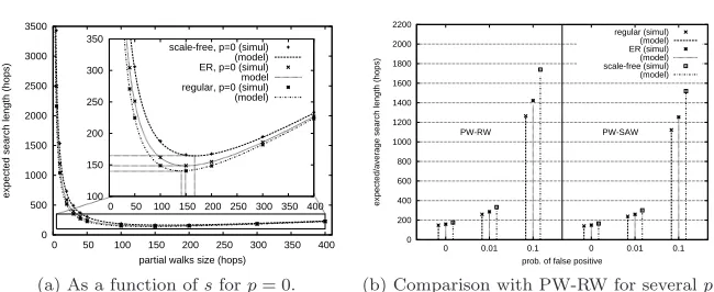
Expected Search Length in PW-SAW. In this section, we compare the analytic results from the model with experimental data from simulations. Figure 4(a) shows the expected search length (Ls) as a function of the size of PWs (s) in
a regular network, an ER network and a scale-free network, for p = 0. The curves in this graph are plotted using Equation 8 and previous equations.
According to the results computed using the PW-SAW model, the mini-mum search lengths occur for values arounds= 141,s= 149 ands= 167 for the regular, ER and scale-free networks, respectively. These values are slightly lower than the ones predicted by the PW-RW model (Figure 2(a)), which were
sopt= 150,157 and 174, respectively.
Both the model curves and the simulation experiments have been computed forw= 5, chosen as a reference value. However, it has been observed that very similar results are obtained if we change the value of w. Furthermore, plots of the model equations for different values ofware coincident. This behavior was also observed for PW-RW (Section 3.2), where we found that the average search length remained almost constant as we increased w. The reason for this is that the probability of the resource being in the chosen PW (pr in
Equation 5) does not depend on the number of PWs in the node.
0 500 1000 1500 2000 2500 3000 3500
0 50 100 150 200 250 300 350 400
expected search length (hops)
partial walks size (hops) 100
150 200 250 300 350
0 50 100 150 200 250 300 350 400
scale-free, p=0 (simul) (model) ER, p=0 (simul) model regular, p=0 (simul) (model)
(a) As a function ofsforp= 0.
0 200 400 600 800 1000 1200 1400 1600 1800 2000 2200
0 0.01 0.1 0 0.01 0.1
expected/average search length (hops)
prob. of false positive regular (simul)
(model) ER (simul) (model) scale-free (simul) (model)
PW-RW PW-SAW
(b) Comparison with PW-RW for severalp.
Fig. 4: Expected search length of PW-SAW in the three networks.
Comparison of performance with respect to choose-first PW-RW. If we com-pare the performance of the proposed search mechanisms, we observe that the reduction in the average search length that PW-SAW achieves with respect to PW-RW for a givenpis largest for the scale-free network, followed by the ER network and then by the regular network. For each network type, the reduction is larger for higherp. Actual values can be found in Table 1(b).
Alternative Analysis for Choose-First PW-RW. This section presents an alter-native analysis for the model of the choose-first PW-RW mechanism described in Section 3.1. This analysis is based on the proof of Theorem 2 for the PW-SAW mechanism. In fact, only the expression forpr(k) (Equation 6), defined
as the probability that a given PW contains the node that holds the resource, needs to be rewritten to reflect the fact that the PW is a simple random walk instead of a self-avoiding random walk. The new expression is:
pr(k) = 1−
µ
1− k
S−krw
·krw−1
krw
¶s
. (9)
The first fraction within the parenthesis in Equation 9 is the ratio of positive endpoints (the degree of the node that holds the resource) and all endpoints in the network (S =P
kk nk) except those of the current node. We usekrw,
which denotes the expectation of the degree of a node visited by a random walk, as an estimation of the degree of the current node. It is obtained as:
krw=
X
k
k·k·Snk = 1
S ·
X
k
k2·nk.
The rest of the equations in the proof of Theorem 2 are valid for this alternative analysis of the choose-first PW-RW mechanism.
5 Check-First PW-RW and PW-SAW
We now present the check-first versions of the PW-RW and PW-SAW search mechanisms, introduced in Section 2. Suppose the search is currently in a node and it needs to pick one of the PWs in that node to decide whether to traverse it or to jump over it. With the new check-first mechanism, it firstchecks the associated resource information ofall the PWs of the node, and then randomly chooses among the PWs with a positive result, if any (otherwise, it chooses among all PWs of the node, as the choose-first version). These check-first mechanisms improve the performance of their choose-first counterparts, since the probability of choosing a PW with the resource increases. This comes at the expense of slightly incrementing the processing power used since several PWs need to be checked, but without incurring extra storage space costs.
A minor additional difference between the algorithms is that in the check-first version, the resource information is registered from the first node (the node next to the current node) to the last node in the PW. This change slightly improves the performance of the new version, since the probability of choosing a PW with the resource increases also in the cases where the resource is held by the last node of the PW.
We have adapted the analysis presented in the proof for Theorem 2 to reflect the new behavior of the check-first PW-RW/PW-SAW mechanisms. Most of the expressions in the analysis of the choose-first versions are still valid for the check-first versions of the mechanisms, so we present here only the equations that need to be modified to reflect the new behavior. That is the case of Equations 7 for the probabilities of choosing a PW with a true positive, false positive, and negative result, respectively. Their counterparts follow. Remember thatiandj represent the number of PWs of the node that return a true positive result and an false positive result, respectively:
ptp=
w
X
i=1
w−i
X
j=0
P(i, j)· i
i+j,
pf p =
w−1
X
i=0
w−i
X
j=1
P(i, j)·i+j j,
pn =P(0,0) = 1−ptp−pf p.
The expression for pr(k) in Equation 9 is still valid for check-first PW-RW.
However, Equation 6 needs to be modified for check-first PW-SAW, since the range of nodes has changed from [0, s−1] to [1, s]:
pr(k) = 1− s
Y
l=1
µ
1− k
S−lk
0 200 400 600 800 1000
0 50 100 150 200 250 300 350 400
expected search length (hops)
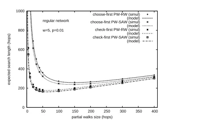
partial walks size (hops) regular network
w=5, p=0.01
choose-first PW-RW (simul) (model) choose-first PW-SAW (simul) (model) check-first PW-RW (simul) (model) check-first PW-SAW (simul) (model)
Fig. 5: Expected search length of choose-first and check-first PW-RW and PW-SAW vs.sin a regular network forp= 0.01 andw= 5.
Finally, Equation 8 also needs modification (for chech-first PW-SAW) in the expectation of trailing steps, for the same reason. The new version, which completes the analysis of the check-first mechanisms, is:
Ls=
1
N
X
k
nk
µ 1
ptp(k)·
(pn(k) +s·pf p(k)) +
s
2
.
Expected Search Length in Check-First PW-RW/PW-SAW. Figure 5 shows the expected search length (Ls) vs. the size of PWs (s) in a regular network
for the four mechanisms presented so far: choose-first PW-RW/PW-SAW, and check-first PW-RW/PW-SAW, forp= 0.01 andw= 5. The check-first mech-anisms achieve a lower minimum than the original choose-first mechmech-anisms, as expected. In fact, the expected search length can be lowered further by in-creasingw, the number of PWs per node, clearly at the expense of increasing the cost of the PWs construction stage. Also interesting is the observation that the minimum expected search length occurs for significantly lowers(sopt
falls from 150 to about 50), meaning shorter PWs in the nodes, which in turn decreases the cost of the PWs construction stage. Regarding the PW-SAW mechanisms, they achieve a slight decrease in the expected search length with respect to the PW-RW mechanisms, both for the check-first and the choose-first versions (already observed in Table 1). Results for the ER and scale-free networks are similar and are omitted here.
6 Future Work
References
1. Lada A. Adamic, Rajan M. Lukose, Amit R. Puniyani, and Bernardo A. Huberman. Search in power-law networks.Physical Review E, 64(046135), 2001.
2. Qin Lv, Pei Cao, Edith Cohen, Kai Li, and Scott Shenker. Search and replication in unstructured peer-to-peer networks. InICS ’02: Proceedings of the 16th international conference on Supercomputing, pages 84–95, New York, NY, USA, 2002. ACM. 3. Shi-Jie Yang. Exploring complex networks by walking on them. Physical Review E,
71(016107), 2005.
4. Christos Gkantsidis, Milena Mihail, and Amin Saberi. Random-walks in peer-to-peer networks: algorithms and evaluation.Performance Evaluation, 63:241–263, 2006. 5. Luis Rodero-Merino, Antonio Fern´andez Anta, Luis L´opez, and Vicent Cholvi.
Perfor-mance of random walks in one-hop replication networks.Computer Networks, 54(5):781– 796, 2010.
6. Van Jacobson, Diana K. Smetters, James D. Thornton, Michael F. Plass, Nick Briggs, and Rebecca Braynard. Networking named content. Commun. ACM, 55(1):117–124, 2012.
7. Andrei Broder and Michael Mitzenmacher. Network applications of bloom filters: A survey. Internet Mathematics, 1(4):485–509, 2004.
8. Atish Das Sarma, Danupon Nanongkai, Gopal Pandurangan, and Prasad Tetali. Dis-tributed random walks.J. ACM, 60(1):2:1–2:31, February 2013.
9. Phouvieng Hieungmany and Shigeo Shioda. Characteristics of random walk search on embedded tree structure for unstructured p2ps. Parallel and Distributed Systems, International Conference on, 0:782–787, 2010.
10. V´ıctor M. L´opez Mill´an, Vicent Cholvi, Luis L´opez, and Antonio Fern´andez Anta. Re-source location based on partial random walks in networks with reRe-source dynamics. InProceedings of the 4th International Workshop on Theoretical Aspects of Dynamic Distributed Systems, TADDS ’12, pages 26–31, New York, NY, USA, 2012. ACM. 11. M. E. J. Newman, S. H. Strogatz, and D. J. Watts. Random graphs with arbitrary
degree distributions and their applications.Physical Review E, 64(026118), 2001. 12. V´ıctor M. L´opez Mill´an, Vicent Cholvi, Luis L´opez, and Antonio Fern´andez Anta.
A model of self-avoiding random walks for searching complex networks. Networks, 60(2):71–85, 2012.
13. L Lov´asz. Random walks on graphs: a survey. InCombinatorics, Paul Erd˝os is eighty, volume 2, pages 1–46. Keszthely, Hungary, 1993.
A Distributions of the Number of Trailing Steps
The proof of Theorem 1 assumes that the distribution of the number of trailing steps in the last PW is uniform between 0 ands−1, corresponding to the cases where the first node/last node in the PW holds the desired resource. Recall that the Bloom filter stores the resources held by thesfirst nodes in the PW, from the node that precomputed the partial walk to the one before its last node (which is included in the partial walks departing from it). We have obtained that distribution from the 106 searches in our experiment for each of the three
networks. Figure 6 shows the results for the regular network whens= 10,s=sopt= 150
ands= 1000. Distributions for the ER and scale-free networks are similar in shape. A slight decrease in the frequency is observed as the number of steps grows. This is due to the fact that the number of trailing steps is essentially the length of the total walk modulus the length of PWs (s). The total walk is a random walk, and its distribution can be obtained approximately by Equation 10.7Since it is a decreasing function, as it is shown
below, the frequency on the left end of an interval of width sis always higher than the frequency on the right end, thus accounting for the observed decrease.
7 The distribution of simple random walk searches has also been obtained experimentally,
99000 99500 100000 100500 101000
0 1 2 3 4 5 6 7 8 9
number of trailing steps
s = 10 frequency
6250 6500 6750 7000 7250
0 40 80 120 149
number of searches
s = sopt = 150 frequency
800 900 1000 1100 1200
0 200 400 600 800 999
s = 1000 frequency
Fig. 6: Distributions of the number of trailing steps in the regular network.
This means that the result provided by Theorem 1 is pessimistic, since the estimated average number of trailing steps is slightly higher than the real one. Results in Section 3.2 have shown that expected search lengths predicted by Equation 1 are very similar to values averaged from simulations data, with larger error for higher values ofs.
The probability distribution of simple random walk searches can be estimated using Equation 10. We show below that it is strictly decreasing, that is: Pi−Pi−1 < 0 for
0≤i <∞:
Pi=
0
@1− i−1 X j=0 Pj 1 A· 1
N−1,fori >0; P0=
1
N. (10)
First, it is shown by induction that 0<Pk
i=0Pi<1 fork≥0 andN >0. It holds trivially
fork= 0. Then, it is also true fork >0 if it holds fork−1:
k X
i=0
Pi=
k−1 X
i=0
Pi+ 1−
k−1 X
i=0
Pi
!
· 1
N−1=
N−2
N−1·
k−1 X
i=0
Pi+
1
N−1 <
N−2
N−1+
1
N−1 = 1.
Next, it is shown that 0< Pi<1 fori≥0 as a corollary of the previous result. It is checked
fori= 0 by inspection. Fori >0, we have thatPi= “
1−Pi−1 j=0Pj
” · 1
N−1. Then:
0<1− i−1 X
j=0
Pj<1, and then : 0< Pi= 0
@1− i−1 X j=0 Pj 1 A· 1
N−1<1.
Finally, it is shown thatPi−Pi−1<0 fori >0. Fori= 1, by inspection. Fori >1:
Pi−Pi−1=
0
@1− i−1 X j=0 Pj 1 A 1
N−1−
0
@1− i−2 X j=0 Pj 1 A 1
N−1=−
Pi−1
N−1.
Since we have shown that 0< Pi−1<1, it follows thatPi−Pi−1<0.
0 2000 4000 6000
0 100 200 300 400
search length w = 2 average
0 2000 4000 6000
number of searches
26.30 % unfinished searches w = 1 average
0 2000 4000
6000 not reused PWs
average
(a)p= 0.
0 1000 2000 3000 4000
0 100 200 300 400 500 600 700
search length w = 2 average 0 1000 2000 3000 4000
number of searches
26.34 % unfinished searches w = 1 average
0 1000 2000 3000
4000 not reused PWs
average
(b)p= 0.01.
Fig. 7: Distributions for non-reused PWs and forw= 1,2 (regular network).
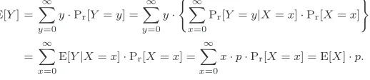
the number of experiments is, in turn, a random variable. Then, from the definition of expectation and the Total Probability Theorem, the expectation ofY is E[Y] = E[X]·p.
E[Y] =
∞ X
y=0
y·Pr[Y =y] =
∞ X y=0 y· (∞ X x=0
Pr[Y =y|X=x]·Pr[X=x] )
=
∞ X
x=0
E[Y|X=x]·Pr[X=x] = ∞ X
x=0
x·p·Pr[X=x] = E[X]·p.
C Searches Based on Reused Partial Walks
We explore here the search length distributions when the total walks are built reusing a limited numberwof PWs per node. How many PWs are necessary for the distributions to be similar to those of non-reused PWs? For the networks considered in our experiment and for the optimal PW size (sopt), we have found that it is enough to have as few astwoPWs.
The extreme case ofonePW yields a significant fraction of unfinished searches, since it is relatively easy to build walks that are loops that do not visit all the nodes. Indeed, if the last node of a PW is a node whose (only) PW has been previously used in that total walk, it will repeatedly take the search to the same place again. However, if one PW is chosen randomly among several ones, the chances of entering a loop are very small.
Figure 7 shows the search lengths distributions in the regular network. The top plots correspond to non-reused PWs. The middle and bottom plots correspond to reusing a single PW or two PW per node, respectively. The shape of the distributions is the same for all
w. However, distributions forw= 1 are lower and the average search length (marked as a vertical bar) is also smaller. This is due to a significant percentage of unfinished searches (about 26%), left out of the histograms, due to loops as explained above. If we focus on the case forw= 2, we note that both the distribution and the average search length are very similar to those of non-reused PWs. Additional experiments with higherwconfirm this observation. As a global measure of the difference between the distributions forw= 2 and for non-reused PWs, we compute themean relative differenceas L 1
90%+1
PL90% l=0
|h2(l)−hnr(l)|
hnr(l) ,
wherehw(l) andhnr(l) are the frequencies of searches with lengthℓwhen usingwpartial
walks and non-reused PWs, respectively. The tail of the distribution is removed, including searches within the 90% percentile (L90%). The mean relative differences forp= 0,p= 0.01