Deterministic and Probabilistic Engineering Cost
Estimating Approaches for Complex Urban Drainage
Infrastructure Capital Improvement (CIP) Programs
Thewodros K. Geberemariam Ph.D., P.E., D. WRE, PMP, QPSWPPP, QCIS, EXW, ENV SP, M.ASCE
P. O. Box 23195 Brooklyn, New York 11202, USA; [email protected]
Abstract:
Accurate and reliable project cost estimates are fundamental to achieve successful municipal capital improvement (CIP) programs. Engineering cost estimates typically represent critical information for key decision makers to authorize and efficiently allocate the necessary funds for construction, budgeting, to generate a request for proposals, contract negotiations, scheduling, etc. for these reasons, cost estimators are using different estimating methods and approaches that allow for required levels of accuracy. As the project’s scope becomes more detailed and the potential risks are identified and/or the project design stage progresses these cost estimates are revised and updated. In this paper, the most common project cost estimation methods and approaches were collected and categorized into two main groups of (1) probabilistic and (2) deterministic methods. Under these groups overall ten different methods were identified and discussed addressing their requirements, advantages, and shortcomings, including the potential risk that can positively or negatively affect the project’s cost outcome. This paper will be a good resource for professionals who are in budget development and/or are seeking to a better understanding of different methods in determining an appropriate base cost margin and produce a meaningful and reliable project cost estimate.
Keywords: Risk management; Deterministic; Probabilistic; Engineering Cost Estimating; Uncertainty; Cost Estimating Methods; Urban Drainage Infrastructure; Capital Improvement (CIP) Programs
Introduction:
The conventional deterministic cost estimation methods for capital improvement projects in most municipal agencies and the local governments are based on preparing a single-point-estimates. A single-point-base-estimate is based on typically on the level of a project’s scope definition and the project design phase, available historical data, current contractor rates and preliminary quotes from sub-contractors and other vendors (Gregory, 2012; Yeo, K. T. 1990). Moreover, to adjust for inflation costs of labor, material, and equipment additional Consumer Price Index (CPI) is added to each cost item every year. This poses a challenge on the accuracy of the project cost estimate and/or budget(s) and may cause cost overruns (Bates et al 2005; Bier, 1997; Gregory, 2012; Reilly et al 2004). Accurately estimating the costs of complex infrastructure projects in the design, and construction phases have typically become a unique challenge for engineers, architects, owners, municipal agencies, and contractors. Complex and technologically advanced projects are usually contained much uncertainty and related challenges than other projects. Therefore, engineering cost estimates must adequately address uncertainty at the preliminary stages of projects where neither the exact quantities nor specific costs or ultimate prices are known. However, dealing with risks and uncertainties are usually a problem (Bates 2005; Sander 2016; Tsagkari et al 2016; Trost and Oberlender 2003).
estimate is gradually reduced (Jensen, 2002; Modarres 2016; Moergli et al 2015;Moergli et al 2015; Ogilvie et al 2012; Reilly 2001; Trost and Oberlender 2003). In the deterministic approach, information about uncertainties and their characteristics such as higher or lower values, ranges of quantities, and potential costs cannot easily be taken into consideration even though this information is generally available or can be estimated. However, the probabilistic approach used best fit probability distributions to model the uncertainties and risk in the cost estimate. The main advantages of the probabilistic cost estimating approaches are its ability to provide insight in the accuracy of the estimate and the impact of uncertainties and risks of cost overruns will be known (Moergli et al 2015; (AASHTO 2009; Booz 2005; WSDOT; 2009; Gregory 2012; Ogilvie et al 2012).
Accuracy of Cost Estimates
The overall purpose of an accurate cost estimate is its use in establishing the budget for a project and as a tool used for scheduling and monitoring and controlling of the project cost. The level of accuracy of engineering cost estimates increases as the project phase progresses and the potential risks are identified. The earlier the estimate in the life of the project the lower its accuracy consequently, assessments of conceptual estimate accuracy are quite low (Bates 2005; Ogilvie et al 2012; Ferry, et al., 1999; AbouRizk, et al., 2002; Christensen and Dysert 2003). Figure-1 below shows the Characteristic curve of accuracy vs. time to make estimates.
Figure-1 Characteristic curve of accuracy vs. time to make estimates
The target cost estimate accuracy set calculated from programmatic data, prior to design generally assumed to be around +/- 30% (Ballard 2013; Gregory 2012; Heldman 2018). However, Experts assert that this variance allows conceptual estimates to be useful for determining feasibility but not for establishing a control budget. Various factors are understood to affect the accuracy of conceptual estimates. list the following factors as primary in conceptual cost estimating of industrial projects, together with their relative impact on estimate accuracy: In general, in schematic and/or preliminary stage (order-of-magnitude) cost estimates accuracy are in between ±20% of actual costs and in detailed estimates are in range of ±5% of actual costs (Council 2009; Dysert and Christensen 2003; Trost and Oberlender 2003; Blank and Tarquin 2005).
Classifications of Cost Estimation Methods
1. Deterministic and Probabilistic Cost Estimating Methods
funded, research and development, operations, etc. The levels of requirements and techniques used are the common characteristics of most project cost estimates (Tsagkari et al 2015; Ogilvie et al 2012; Shane et al 2015; WSDOT 2009; Trost and Oberlender 2003). These includes (1) Status of Project life cycle, (2) the detail information available, (3) cost estimation methods (e.g., parametric vs. definitive), and/or (4) Constraints and other estimating variables such as time (Trost and Oberlender 2003; Reilly et al 2004). Preparing cost estimate also depending on the purpose, level of planning, and/or design, as well as the project type, size, complexity, circumstances, schedule, and location (Tsagkari et al 2015, 2016). These methods can fall into categories such as parametric, historical bid-based, unit cost/quantity bid-based, range, and probabilistic risk-based estimates (Burak 2010; Moergli et al 2015; Rush and Roy 2000; Gregory 2012). Figure-2 below shows, the two major Classifications of Cost Estimation approaches namely deterministic and probabilistic method.
Figure-2 Classifications of Cost Estimation Methods
Generally, in the deterministic approach, information about uncertainties and their characteristics such as higher or lower values, ranges of quantities, and potential costs cannot easily be taken into consideration even though this information is generally available or can be estimated (AACE International 2003; Bates 2005; Bajaj et al 2002; Lemmens 2016; Ostwald 1974; Qian and Ben-Arieh 2008). However, the probabilistic approach used best fit probability distributions to model the uncertainties and risk in the cost estimate (Anderson et al 2007; Bier 1997; Jensen 2002; Bier 1997; Evans and Peck 2008). The main advantages of the probabilistic cost estimating approach is its ability to provide insight into the accuracy of the estimate and the impact of uncertainties and risks of cost overruns Bier 1997; Elkjaer 2000; Modarres 2016; Moergli et al 2015 ;Chou 2011; Sander 2016; Shane et al 2015; Trost and Oberlender 2003).
The fundamental difference between these two cost estimation approaches (probabilistic and deterministic) is that by using the probabilistic cost estimation approach, we are enabling explicitly model the uncertainties and risk associated with it using appropriate statistical distributions (Gregory 2012; Touran 2006; Kermanshachi et al 2018; WSDOT July 2010; Whitesides 2005; Ostwald 1974).
1.1 Deterministic cost estimating
Under this category, Parametric, Detailed, Comparative, (Unit, cost, and Power law and sizing method), and Factored Estimates methods have been discussed below:
I. Parametric cost estimating (top-down estimating)
This method is generally used during the earliest stage of the project (Qian and Ben 2008). However, it also can be used to establish a baseline at any stage, where the comparison or validation of other estimating methods are needed or estimation of the use of resources required to perform for a new
Cos
t Es
tima
tion Methods
Deterministic
project (Roy and Rush 2000, 2001; Fad et al 1998; Bajaj et al 2002; Black 1984). This model has a mathematical representation of the cost estimating relationships (CERs) that able to predict and provides a logical correlation between the physical and functional characteristics of a project (Dysert 2008; Ostwald 1974; Ayyub and McCuen 2016; Qian and Ben 2008).
A particular cost or price can be established and estimated using cost estimating relationships (CERs) with an independent variable. The cost estimating relationship (CER), mathematical ratio or equation can be developed using an independent variable that demonstrates a measurable relationship between contract cost and price (Ayyub and McCuen 2016; Qian and Ben 2008). It usually derived from regression analysis of historical systems or subsystems. Equation (1) and (2) below are the associated linear and nonlinear form of cost estimation relationships (CER). The equations are called cost estimating relationships (CER's) framework. The CER uses quantitative techniques to quantify a relationship between an independent variable and contract cost or price (Ostwald 1974; Ostwald 1974; Bajaj 2002; Black 1984; Reilly et al 2001, Reilly 2004; Qian and Ben-Arieh 2008; Kermanshachi et al 2018).
𝑇 = 𝑃 𝑃 … … … (1)
Where:
𝑻𝑪 = Total Cost
𝑷𝑪𝑹 = parameter cost ratio
𝑷𝑰 = parameter of an interest
Equation two for CER with associated nonlinear form cost estimation relationships
𝑇 = 𝑃 𝑃 … … … (2)
Where:
𝑷𝑰 = parameter of independent variable of interest
𝐧𝐢 = exponent used to transform 𝑷𝑰
The exponential factors (E.q-2) used to transform and normalize the temporal effects of cost including an inflation, rapid increases of material cost, and for an independent variable and other metrics. In general, Parametric cost estimating can also be incorporated with probabilistic estimating to form range estimating that predict uncertainties and potential risks (Roy and Rush 2000; Kermanshachi et al 2018; Bajaj 2002; Black 1984, Gregory 2012; Ogilvie et al 2012; WSDOT 2010).
Table-1 Parametric Cost Estimating Method
Advantage Disadvantage Requirement
Relatively quick and accurate way to estimate costs
Documentation of Cost Estimating Relationships (CERs) can be difficult
Sufficient historical data for statistical analyses
Reduced likelihood of serious cost overruns
Reduced cost of preparing project proposals
Historical data must be available Database Multiple decision options for project
managers
Improper use of CERs can lead to serious estimating errors Model can be used as basis for
uncertainty and risk analyses
Maintenance of database with historical data
Easy to combine with other estimating methods
Periodically updated to capture the most current cost, technical, and programmatic data.
II. Detailed cost estimating /Bottom-up/ Analytical Estimating Method
The detailed cost estimating requires is the most accurate estimating technique when, the project is decomposed into manageable tasks, or when works breakdown structure is available (Chou et al., 2009; Chou 2011). A work breakdown structure is used to divides project deliverables into a series of work packages and each work package comprised of a series of tasks (Dell’Isola 2003; Rolstadås 2004;Rush and Roy 2000; Sonmez 2004). During detailed cost estimate, the project teams of cost estimators work with engineers, Architects etc. to complete each itemized task and work packages and develop the total detailed cost estimate for the entire proposed project (Government Accountability Office, 2009). The cost estimator’s quantity estimates have to be validated by the professional engineers to make sure this cost estimation process is leads to a consistent and reproducible result (NASA, 2008;Rosse 1970; Kumari and Pushkar 2013). Equation-3 below is the general mathematical formula. However, this method is different for each project.
𝑇 = 𝑞 (𝑀 + 𝑊 + 𝐿 ) + 𝐼 𝑈𝐶 … … … (3)
Where:
𝑻𝑪 = Total Cost
𝒒𝒊 = quantity of work
𝑴𝒊 = Unit material cost
𝑾𝒊 = Unit Wage rate
𝑳𝒊 = Unit Labor Rate
𝑰𝒋 = measure of work in indirect cost elements
𝑪𝒋 = Unit cost of in indirect elements
Certainly, the detailed cost estimating is the most accurate and provides insight into the major cost contributors, all cost components and make sure nothing can be overlooked (Clark and Lorenzoni 1996; NASA, 2008). However, it can also be time-consuming, and requires a lot of effort to establish especially in large and complex projects with numerous work breakdown structure components (Dell’Isola 2003; Burns et al 1993; NASA, 2008; Shen and Issa 2010).
Table-2 Detailed Cost Estimating Method
Advantage Disadvantage Requirement
A greater level of confidence Very high accuracy possible
More time needed to develop the estimate
All cost components are taken into account
more costly to develop than relationship estimating
Work Breakdown Structure Nothing can be overlooked Historical data must be available Additional ‘sanity’ check or
benchmark Parts of the estimates can be reused Project’s scope must be determined
and understood considerably Actual cost data of ongoing project
can be used as predictor for future
Confidence level difficult to determine
III. Comparative cost estimating/Analogous Estimating Method
The comparative estimating method can be used to make a quick comparison when a new project is similar to another project recently completed. During this process the major cost components that were used on previous similar projects and direct and recent experience is needed (Lester, 2013; Griffith et al 2014). Adjustment shall be made on the proposed cost estimate factoring the differences in project size and complexity, performance requirements, duration, location and available technology (Government Accountability Office, 2009; Nijkamp and Ubbels 1999). This relation factors are not usually linear. Cost capacity factors and economies of scale are the main factors that determine the nonlinear form of cost estimation relationships (CER) (Akintoye 2000;Burke, 2003; Flyvbjerg et al 2002). Commonly used technique for preliminary design stage cost estimates are Unit Method, cost indexes, Cost-Capacity Equation or power law and sizing model, and Factored Estimates (Wilmot and Cheng 2003). The general mathematical Cost estimate equations are presented below.
I. Unit Method
𝑇 = U ∗ 𝑁 … … … (4)
Where:
𝑻𝑪 = Total Cost
U= per unit cost
N= quantity of work
II. Cost Indexes
Cost Index (CI) is the ratio of cost to date versus cost in the past. The CI change in cost over time to account the impact of inflation and it is dimensionless (William 1994). The general mathematical formula used to calculate the total Cost estimate is:
𝑇 = 𝐶 𝐼
𝐼 … … … (5)
Where:
𝑻𝑪 = Estimated total cost of present time
𝑪𝟎 = Cost at previous time
𝑰𝟎 = Index value at base time 0
III. Cost-Capacity Equation or Power Law and Sizing Model
The general mathematical formula used to calculate the total Cost estimate is:
𝐶 = 𝐶 𝑄
𝑄 … … … . . (6)
Where:
𝑪𝟏 = Cost at Capacity 𝑸𝟏
𝑪𝟐 = Cost at Capacity 𝑸𝟐
x= Correlating Exponent
Where:
X = 1, relationship is linear
X < 1, economies of scale (larger capacity is less costly than linear)
X > 1, diseconomies of scale
Cost-Capacity Combined with Cost Index: Multiply the cost-capacity equation by a cost index to adjust for time differences and obtain estimates of current cost (in constant-value dollars)
𝐶 = 𝐶 𝑄 𝑄
𝐼
𝐼 … … … (7)
Some of the advantages of this method are its ability to generate quick, easily, very accurate and understandable cost estimate for the proposed project, especially when the proposed project has minor deviations from an appropriate comparative similar past project that has been completed(Akintoye 2000;Burke, 2003; Flyvbjerg et al 2002).The shortcomings of this method are its dependent on a single data point, its requirement of normalization in order to create baseline and ensure a good accuracy of the estimate, and also the difficulties of finding an appropriate comparative data for similar past project and experts to make judgment to adjustment factors(Edwards et al 2000, William 1994).
Table-3 Comparative Cost Estimating Method
Advantage Disadvantage Requirement
Easy to generate and estimate, provided historical data is available.
Uncertainty due to subjective evaluations made by estimator.
Requires analogous product and program data.
Provides better credibility than plain detailed estimating. Can be used early in project even if scope of the project is not complete
Difficult to apply for differences in scope of work, design, configuration and number of aircraft or aircraft programs.
Requires a detailed program and technical definition of the analogous system as well, as the system being estimated.
Quick and reasonable accuracy for similar systems, or end items. Estimate is easy to understand
Once the technical assessment has identified the analogous system, actual cost data on that system must be obtained.
Good accuracy for similar systems if comparative and recent data is available
Accuracy is limited, Cost impacting factors have to be determined, and Normalization required
Comparison factors
IV. Ratio or Factored Estimates Method
In this method, scaling relationships used to forecast the cost of new project when historical and component data are available from similar project (Christensen and Dysert 2003). However, this scaling relationships does not includes economical factor, location and the timing of the work. Generally, this method is used in estimating total plant cost in the processing industries. Both direct and indirect costs can be included (Humphreys 1995; Dysert 2003; Lemmens 2016; Clark and Lorenzoni 1996). The general mathematical formula used to calculate the total Cost estimate can be expressed as:
𝑇 = 𝐶 𝑓 ∗ 𝐶 ∗ (𝑓 + 1) … … … . . … … … (8)
Where:
𝑪𝑬 = The total cost of major equipment item
𝒇𝒊 = Overall cost factor and can be determined using two basis
Delivered equipment cost including purchase cost of major equipment
Installation cost
(𝒇𝑰+ 𝟏) = The cost factor (commonly the sum of a direct cost component and an indirect
cost component) for I = 1, 2… n components, including indirect costs
1.2 Probabilistic cost estimating Method
The probabilistic cost estimating techniques focus on the risks and uncertainties involved in the project and attempt to quantify the project cost variability based on one or more parameters. It addresses the concerns regarding the chance of exceeding a particular cost in the range of possible costs, the possible amount of the cost overrun, and the different types of uncertainties and how they drive cost (Anderson et al. 2007; Jensen 2002; Modarres 2016; Moergli et al. 2015; Bier 1997; Shane et al. 2015; Trost and Oberlender 2003; WSDOT 2009, 2010). The probabilistic cost estimating techniques uses probability distribution to consider range estimation rather than point estimates to reflect the different outcomes (Elkjaer, 2000; (Clark and Lorenzoni 1996; Garvey 2000; Chou et al. 2009; FHWA January 200). The Expected value, Variance, Covariance and the Central Limit are some of the key aspects of the mathematical application of probabilistic cost estimating techniques.
I. Expected value
The expected value of a cost parameter can be defined as the weighted average of all possible values. The term expected value in essence means the same as the often used term average (Ostwald 1974). The expected value equals:
𝐸(𝑋 ) = 𝜇 = 𝑥 𝑓(𝑥) 𝑑𝑥 … … … . . … … . (9)
𝒇(𝒙) = The probability density functions of cost parameter 𝒊. If all cost parameters of 𝒊 are correlated such that 𝒀 = 𝒙𝟏+ 𝒙𝟐, then
𝐸(𝑌) = 𝐸(𝑋 ) + 𝐸(𝑋 ) … … … . … … . . … (10)
The variance in this case is given by 𝛿𝑌 = 𝛿 + 𝛿 + 2𝛿, in this formula 𝛿, is the covariance of
random variables of 𝑥 𝑎𝑛𝑑 𝑥 . If the random variables are independent then 𝛿, is equal to zero. If
the total cost is the product of independent, continuous, random variables, such that= 𝑥 ∗ 𝑥 , then
𝐸(𝑌) = 𝐸(𝑋 ) + 𝐸(𝑋 ) … … … . . … … (11) 𝛿𝑌 = 𝑋 𝛿 + 𝑋 ∗ 𝛿 + 𝛿 𝛿 … … … . . … … (12)
II. Variance
In probability theory, variance gives a measure of how much the values of a function of a random variable x vary as we sample x from a probability distribution. When the variance is low, values of f(x) cluster around its expected value. The square root of the variance is known as the standard deviation and usually indicated with the symbol σ(Beck and Arnold 1977; Moergli et al. 2015; Jensen 2002).
III. Covariance
Covariance measures how two values are linearly related, as well as scale of variables. Calculating correlation is an important to analyze the correlation between two or more cost components that can have a large impact on the degree of risk associated with using the variance (Touran, 1993; Wall, 1997; Yang, 2005; Jensen 2002).If two random variables have no correlation with covariance equal to zero they are called independent (Beck and Arnold 1977). The covariance can be high absolute, positive, zero or negative. High absolute values of covariance means values change very much & are both far from their mean. Positive value means both variables take relatively high values far from mean. Negative value means one variable takes on high values & another takes low values (Yang, 2005; Jensen 2002).
The formula that can be used to calculate the covariance of two random variables X and Y, denoted by 𝑪𝒐𝒗(𝑿, 𝒀)is defined as:
𝐶𝑜𝑣(𝑋, 𝑌) = 𝐸(𝑋𝑌) − 𝜇 𝜇 … … … . … … … (13)
Therefore, the Pearson’s correlation coefficient between data sets X and Y can be calculated:
𝑟 = ∑ (𝑋 − 𝑋)(𝑌 − 𝑌) ∑ (𝑋 − 𝑋) ∑ (𝑌 − 𝑌)
… … … . (14)
Where: r = Pearson’s correlation coefficient
𝑿 = Mean of data set X
𝒀 = Mean of data set Y IV. Central Limit Theorem
approximately the normal distribution with mean µ and standard deviation √σ n , where µ and σ are the mean and standard deviation of the population from where the sample was selected (Shaheen et al. 2007(Dekking et al. 2005; Diekmann, 1983 ;). In order to be able to give lower and upper bounds on the total cost we use confidence limits. A confidence limits are the probability that the interval estimate will include the lower and upper bound of cost parameter (Shaheen et al. 2007).
𝑳𝑩𝑻𝑪 = 𝑬𝑻𝑪 − 𝒁 ∗ 𝝈 … … … . (𝟏𝟓) 𝑼𝑩𝑻𝑪 = 𝑬𝑻𝑪 + 𝒁 ∗ 𝝈 … … … . (𝟏𝟔)
Where: 𝑳𝑩𝑻𝑪 =Lower bound on Total Cost
𝑼𝑩𝑻𝑪= Upper bound on Total Cost
𝑬𝑻𝑪 =Expected Total Cost
𝝈 = Standard Deviation
Z= is determined by the confidence level using the standardized Normal distribution
Table-5confidence level using the standardized Normal distribution
Confidence Level Value of Z
90% 1.28
95% 1.65
98% 2.05
99.9% 3.09
1.2 Probability distributions
Different cost parameters coupled with several simple probability distributions are useful in many engineering cost estimation modeling and risk analysis. Normal, Lognormal, Beta, Triangular and Weibull are typical probability distributions that are commonly used in the construction industry (Chou et al., 2009; Anderson et al. 2007; Jensen 2002; Modarres 2016; Moergli et al. 2015; Bier 1997; Shane et al. 2015; Trost and Oberlender 2003; WSDOT 2009, 2010).below are summary of discussion together with the probability density function (PDF), the cumulative density function (CDF), the expected value (E(X)) and the variance (Var(X)) of each distributions.
I. Uniform distribution
The uniform distribution is a continuous probability distribution the assumption: the random event is equally likely in an interval. It is defined by two parameters, the minimum possible value (a) and the maximum possible value (b).
A variable X is said to be uniformly distributed if the density function is:
𝒇(𝒙) =
𝟏 𝒃 𝒂
𝟎 𝒇𝒐𝒓 𝒐𝒓 − ∞ < 𝒂 ≤ 𝒙 ≤ 𝒃 < ∞ … … … . . … … (𝟏𝟕)
Figure -3 the graph of a uniform distribution
The mean and variance of X following a uniform distribution is:
𝐸(𝑋) =(𝑎 + 𝑏)
2 … … … (18) 𝑉(𝑋) =(𝑏 − 𝑎)
12 … … … (19)
The standard uniform density has parameters a = 0 and b = 1, so the PDF for standard uniform density is given by:
𝑓(𝑥) = 0, 𝑜𝑡ℎ𝑒𝑟𝑤𝑖𝑠𝑒 … … … . .1, 0 ≤ 𝑥 ≤ 1 (20)
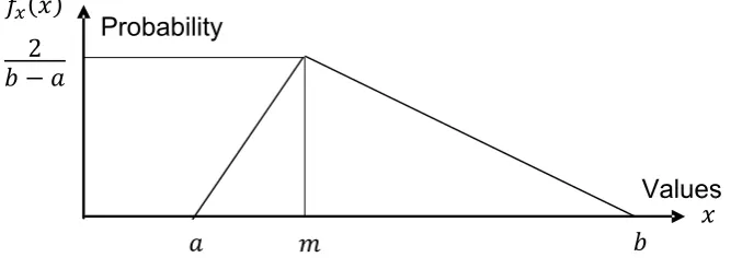
II. Triangular Distribution
In this method it is assumed that a Triangular or Beta distribution can be used to describe each item T (a, m, b). This means that the user gives an optimistic estimate a, a most likely estimate m and finally a pessimistic estimate b (Garvey 2000; Garvey et al. 2016; Shane et al. 2015; Ayyub and McCuen 2016). A Triangular distribution might look like this:
Figure -4 Sample of triangular distribution (a) =lowest (b) = highest, and (M) = most likely values
The PDF of the triangular distribution is given by:
Probability
Values
𝑎
𝑚
𝑏
𝑓 (𝑥)
𝑥
2
𝑓 (𝑥) = ⎩ ⎪ ⎨ ⎪
⎧ 2(𝑥 − 𝑎)
(𝑏 − 𝑎)(𝑚 − 𝑎) 𝑖𝑓 𝑎 ≤ 𝑥 ≤ 𝑚 2(𝑏 − 𝑥)
(𝑏 − 𝑎)(𝑚 − 𝑎) 𝑖𝑓 𝑚 ≤ 𝑥 ≤ 𝑏
… … … . … (20)
The cumulative probability distribution of the triangular distribution is given by
𝑓 (𝑥) = ⎩ ⎪ ⎪ ⎨ ⎪ ⎪
⎧ 0 𝑖𝑓 𝑥 < 𝑎(𝑥 − 𝑎) (𝑏 − 𝑎)(𝑚 − 𝑎) 𝑖𝑓 𝑎 ≤ 𝑥 < 𝑚 1 −(𝑏 − 𝑎)(𝑏 − 𝑚)(𝑏 − 𝑥) 𝑖𝑓 𝑚 ≤ 𝑥 < 𝑏
1 𝑖𝑓 𝑥 ≥ 𝑏
… … … . . (22)
The expected value is given by:
𝐸(𝑋) =𝑎 + 𝑚 + 𝑏
3 … … … . … … (23)
The variance is given by:
𝑉(𝑋) =𝑎 + 𝑚 + 𝑏 + 𝑎𝑏 + 𝑎𝑚 + 𝑚𝑏
18 … … … . … … . (24)
The standard deviation is given by:
𝛿 = 𝑎 + 𝑚 + 𝑏 − 𝑎𝑚 − 𝑎𝑏 − 𝑚𝑏
18 … … … . . (25)
III. Beta Distribution
One of its most common uses of this distribution is to model uncertainty and bounded continuous random variables based on expert’s judgment. . The Beta (α, β) distribution is a continuous probability that is defined by two shape parameters α and β (Garvey 2000 b, Garvey et al. 2016; Erkoyuncu et al. 2013; Ayyub and McCuen 2016). The general formula for the probability density function of the beta distribution is:
𝑓(𝑥) = 𝐻 − 𝐿1 Γ(𝛼)Γ(𝛽)Γ(𝛼 − 𝛽) 𝐻 − 𝐿𝑥 − 𝐿 𝐻 − 𝑥𝐻 − 𝐿 𝐿 < 𝑥 < 𝐻 = 0 𝑜𝑡ℎ𝑒𝑟𝑤𝑖𝑠𝑒
… … … (26)
Figure-5 Sample of beta distribution
Most schedule or cost estimates follow right skewed pattern. The value of 𝜶 𝒂𝒏𝒅 𝜷 can be determined using Beta-PERT (L, H, M) Distribution using L, M, and H to calculate the expected value mean and standard deviation as (Garvey 2000 b, Garvey et al. 2016; Erkoyuncu et al. 2013; Ayyub and McCuen 2016):
𝐸(𝑋) = 𝜇 =(𝐿 + 4𝑀 + 𝐻)
6 𝑉𝑎𝑟 (𝑋) =
(𝐻 − 𝐿)
36 𝜎 =
(𝐻 − 𝐿)
6 … … . . (27)
𝛼 𝑎𝑛𝑑 𝛽 = ⎩ ⎪ ⎨ ⎪
⎧𝛼 = (𝜇 − 𝐿) (𝐻 − 𝐿)∗
(𝜇 − 𝐿)(𝐻 − 𝜇)
𝜎 − 1
𝛽 =(𝐻 − 𝜇)(𝜇 − 𝐿) ∗ 𝛼
… … … (28)
Or, from the expected value (µ) and the distribution P (L, M, H) the parameters α and β can be derived by
𝛼 𝑎𝑛𝑑 𝛽 = ⎩ ⎪ ⎨ ⎪
⎧𝛼 =(𝜇 − 𝐿)(2𝑀 − 𝐿 − 𝐻) (𝐻 − 𝐿)(𝑀 − 𝜇) 𝛽 =𝛼(𝐻 − 𝜇)
(𝜇 − 𝐿)
… … … . … … (29)
Where: 𝛼 > 0, 𝛽 > 0 (L), lowest
(H) Highest and
(M) Most likely values
IV. Normal Distribution
The normal distribution is a continuous probability distribution and it has two parameters, µ and σ and is denoted N (µ, σ). Here µ is its mean, 𝜹𝟐 its variance, and σ is its standard deviation (Ayyub and McCuen 2016; Bates et al. 2005;Bier 1997; Dysert 2003; Edwards et al. 2000; Erkoyuncu et al. 2013). The normal distribution is a continuous distribution with probability density function of:
𝑓 (𝑥) = 1
𝛿√2𝜋𝑒 … … … . . . (30)
The cumulative probability distribution of the normal distribution is given by: 0
0.5 1 1.5 2 2.5 3
0 0.25 0.5 0.75 1
X
f(x
𝑓 (𝑥) = 𝑃(𝑋 ≤ 𝑥) = 1
𝛿√2𝜋𝑒 … … … . (31)
The expected value is given by
𝐸(𝑋) = 𝜇 … … … . (32)
The expected value is given by
𝑉𝑎𝑟(𝑋) = 𝛿 … … … . (33)
Figure-6 Sample of standard normal distribution
V. Lognormal Distribution
The log-normal distribution is the probability distribution where the natural log of the sample values has a normal distribution. The probability density function (pdf) is given by ln (N (µ, σ2))
(Ayyub and McCuen 2016; Garvey et al. 2016; Moergli et al 2015).
𝑓(𝑥) = 1
𝑥𝛽√2𝜋 𝑒 − 1 2
ln 𝑥 − 𝛼
𝛽 … … … (34)
Where: α is the mean of ln(x) and β is the standard deviation of ln(x). These are related to the mean and standard deviation of random variable x (µ and σ respectively) as follows:
𝜇 = 𝑒 𝛼 +1
2𝛽 … … … . . (35) 𝛿 = 𝑒 2𝛼 + 𝛽 (𝑒 𝛽 − 1) … … … . . . (36) 𝛼 = ln 𝜇 −1
2𝑖𝑛 𝛼
𝜋 + 1 … … … . . . (37)
µ - σ
µ
µ + σ
µ + 2σ
µ + 3σ
µ - 2σ
µ - 3σ
68%
95%
𝛽 = 𝑙𝑛 𝛼
𝜋 + 1 … … … . … … … . . … . … . (38)
Figure-7 sample of lognormal distributions
P is the cumulative probability function (CDF) of the log normal distribution, is given by
𝑃(𝑥 ≤ 𝑋) = 1
𝑥𝛽√2𝜋 𝑒 − 1 2
ln 𝑥 − 𝛼
𝛽 𝑑𝑥 … … … . . … … … . . (39)
Note that F is the cumulative probability function (CDF) for the standard normal probability distribution
𝑃(𝑥 ≤ 𝑋) = 𝐹 𝑙𝑛 𝑋 − 𝛼
𝛽 … … … . … … . (40)
The Expected value is given by:
𝐸(𝑋) = 𝑒 … … … . . … … … . (41)
The variance is given by:
𝑉𝑎𝑟(𝑋) = 𝑒 − 1 𝑒 … … … . (42)
VI. Weibull distribution
Generally, the Weibull distribution is one of the most commonly used statistical model for project cost estimations and many other applications. The Weibull Distribution (1939) was first published to represent the probability of failure and has proven to be extremely useful for data analysis in many engineering applications such as aerospace, automotive, electric power, nuclear power, medical, dental, electronics and every industry (Ayyub and McCuen 2016; Garvey et al. 2016; Moergli et al 2015; Kujawski et al. 2004; Chou 2011). A continuous function X is said to have a Weibull distribution with parameters δ > 0 and β > 0 if the PDF of X is:
𝑓(𝑥) = 𝛽 𝛿
𝑥
𝛿 𝑒 −
𝑥
The Expected value is given by:
𝜇 = 𝐸(𝑋) = 𝛿Γ 1 + 1
𝛽 … … … . . … … … . … . (44)
The Variance is given by:
𝛿 = 𝑉(𝑋) = 𝛿 Γ 1 + 2
𝛽 − 𝜇 , 𝑤ℎ𝑒𝑟𝑒 𝑋~ 𝑊𝑒𝑖𝑏𝑢𝑙𝑙(,) … . . … … … . … … … . (44)
The cumulative probability function (CDF) for the standard Weibull (δ,β) probability distribution is given by:
𝐹(𝑥) = 1 − 𝑒 − 𝑥
𝛿 , 𝐹(𝑥) = 0, 𝑓𝑜𝑟 𝑥 ≤ 0 … … … . … . … … . (46)
Figure-8 sample of Weibull distribution
Table-6 Probabilistic Cost Estimating Method
Advantage Disadvantage Requirement
Probability of cost overrun is insightful and defined as opportunities or threats
Additional analysis that requires additional effort
Probability distribution of cost components based on historical data or experience
Improved reliability of the estimate Determining probability distributions may be difficult
Software to run Monte Carlo Simulation
Range of outcomes is available Uncertainties and risks are mapped and quantified
Conclusion
methods, (4) Ratio or Factored estimates method, and (1) Uniform distribution methods, (2) Triangular distribution methods, (3) Beta distribution method, (4) Normal Distribution methods, (5) Lognormal distribution methods, and (6) Weibull distribution method. Overall ten different methods were identified and discussed under these categories to addresses their advantages and shortcomings including the potential risk that can positively or negatively affect the project’s cost outcome, with the intent of ensuring that this paper will be a good resource for professionals who are in budget development and/or seeking to maximize and produce a meaningful and reliable project cost estimate for their projects.
Table-7 Pros and Cons of Deterministic and Probabilistic Cost Estimations Methods
Deterministic Probabilistic
Pros Cons Pros Cons
Varity of techniques may be used including engineering judgement, factor of safety, etc .
Does not determined residual risk. Unknown risk, can be inconsistent between sites. For areal sources, selection of deterministic event is uncertain
known risk, handles areal sources in a consistent way
more complex, still wide-spread misunderstanding
simple to use , Doesn’t rely on statistics, Maintains dependencies
away from measured or interpreted data, Not statistical,
Uses impartial statistical rules, Exhaustive cases can be run,
Needs probabilistic thinking & understanding Needs software support One single figure
Well-known & accepted Quick Can be performed “manually”
No probability information of single value No Value at Risk information More often than not on the unsafe side (high, unknown probability of cost overruns)
All potential risks are included, best estimation assumptions, and follow well established methodology.
Time consuming
Good accuracy for similar systems if comparative and recent data is available
Accuracy is limited, Cost impacting factors have to be determined, and Normalization required
Multiple and common cause of failures can be easily assessed and addressed at the early stage
Comparison factors
Reference:
1. AACE International 2003, “Cost Estimate Classification System”
http://www.aacei.org/technical/rps/18r-97.pdf
2. AbouRizk, S., & Mohamed, Y. (2002, December). CEPM 1: optimal construction project
planning. In Proceedings of the 34th conference on Winter simulation: exploring new frontiers (pp.
1704-1708). Winter Simulation Conference.
3. Akintoye, A. (2000). Analysis of Factors Influencing Project Cost Estimating Practice.
Construction Management and Economics, 18(7) 77-89
4. Anderson, S. D., Molenaar, K. R., & Schexnayder, C. J. (2007). Guidance for cost estimation and
management for highway projects during planning, programming, and preconstruction (Vol. 574).
5. Ayyub, B. M., & McCuen, R. H. (2016). Probability, statistics, and reliability for engineers and
scientists. CRC press.
6. Bajaj, A., Gransberg, D. D., & Grenz, M. D. (2002). Parametric estimating for design
costs. AACE International Transactions, ES81.
7. Bakhshi, P., & Touran, A. (2012). A Method for Calculating Cost Correlation among
Construction Projects in a Portfolio. International Journal of Architecture, Engineering and
Construction, 1 (3), 134-141.
8. Bakhshi, P., & Touran, A. (2014). An overview of budget contingency calculation methods
in construction industry. Procedia Engineering, 85, 52-60.
9. Ballard, G., & Pennanen, A. (2013). Conceptual estimating and target costing. In Proc. 21st
Ann. Conf. of the Int’l. Group for Lean Construction (pp. 31-2).
10. Bates, J., Burton, C. D. J., Creese, R. C., Hollmann, J. K., Humphreys, K. K., McDonald Jr, D.
F., & Miller, C. A. (2005). Cost estimate classification system–as applied in engineering,
procurement, and construction for the process industries.
11. Beck, J. V., & Arnold, K. J. (1977). Parameter estimation in engineering and science. James Beck.
12. Bier, V. M. (1997). An overview of probabilistic risk analysis for complex engineered
systems. Fundamentals of risk analysis and risk management, 67.
13. Black, J. (1984). Application of parametric estimating to cost engineering. AACE transactions,
B-10.
14. Blank, L., & Tarquin, A. (2005). Engineering economy. McGraw-Hill.
15. Burak Evrenosoglu, F. (2010). Modeling Historical Cost Data for Probabilistic Range
Estimating. Cost Engineering, 52(5), 11.
16. Burns, T. J., Page, E. C., Gregory, R. A., & Pryor, G. M. (1993). U.S. Patent No. 5,189,606.
Washington, DC: U.S. Patent and Trademark Office.
17. Chou, J. S. (2009). Generalized linear model-based expert system for estimating the cost of
18. Chou, J.-S. 2011. ‘Cost Simulation in an Item-Based Project Involving Construction
Engineering and Management.’ International Journal of Project Management 29 (6): 709–17.
19. Christensen, P., & Dysert, L. R. (2003). AACE international recommended practice no.
17R-97 cost estimate classification system. AACE International, USA.
20. Clark, F., & Lorenzoni, A. B. (1996). Applied cost engineering. CRC Press.
21. Council, P. S. R. (2009). Benefit-Cost Analysis: General Methods and Approach. The Council.
22. Dell’Isola, M. D. (2003). Detailed cost estimating. Excerpt from Archit. Handb. Prof. Pract,
1-13.
23. Diekmann, J. E. (1983). Probabilistic estimating: mathematics and applications. Journal of
Construction Engineering and Management, 109(3), 297-308.
24. Dysert, L. R. (2003). Sharpen your cost estimating skills. Cost Engineering, 45(6), 22.
25. Edwards, D. J., Holt, G. D., & Harris, F. C. (2000). A comparative analysis between the
multilayer perceptron “neural network” and multiple regression analysis for predicting
construction plant maintenance costs. Journal of Quality in Maintenance Engineering, 6(1),
45-61.
26. Elkjaer, M. (2000). Stochastic budget simulation. International Journal of Project Management, 18(2), 139-147.
27. Erkoyuncu, J. A., Durugbo, C., Shehab, E., Roy, R., Parker, R., Gath, A., & Howell, D. (2013).
Uncertainty driven service cost estimation for decision support at the bidding
stage. International Journal of Production Research, 51(19), 5771-5788.
28. Evans and Peck Report for Department of Infrastructure, Transport, Regional Development
and Local Government (2008), Best Practice Cost Estimation for Publicly Funded Road and
Rail Construction, viewed 10 Jan 2013, http://www.nation
29. Fad, B., Summers, R., DeMarco, A., Geiser, T., Walter, J., Chackman, B., & King, E.
(1998). U.S. Patent No. 5,793,632. Washington, DC: U.S. Patent and Trademark Office.
30. FHWA (January 2004). Guidelines on Preparing Engineer’s Estimates, Bid Reviews and
31. Flyvbjerg, B., Holm, M. S., & Buhl, S. (2002). Underestimating costs in public works
projects: Error or lie?. Journal of the American planning association, 68(3), 279-295.
32. Garvey, P. R., Book, S. A., & Covert, R. P. (2016). Probability methods for cost uncertainty
analysis: A systems engineering perspective. Chapman and Hall/CRC.
33. Grayson, J., Nickerson, J., & Moonin, E. (2015). Partnering through Risk Management: Lake Mead Intake No. 3. Risk Management Approach. RETC June.
34. Gregory, N. (2012) Improving Cost Estimation with Quantitative Risk Analysis. Vose
Consulting, www.voseconsulting.com.
35. Griffith, A., Stephenson, P., & Watson, P. (2014). Management systems for construction.
Routledge.
36. Heldman, K. (2018). PMP: project management professional exam study guide. John Wiley &
Sons.
37. Humphreys, K. K. (1995). Basic cost engineering. CRC Press.
38. Jensen, U. (2002). Probabilistic risk analysis: foundations and methods.
39. Kermanshachi, S., Anderson, S., Molenaar, K. R., & Schexnayder, C. (2018). Effectiveness
Assessment of Transportation Cost Estimation and Cost Management Workforce
Educational Training for Complex Projects. In International Conference on Transportation and
Development(p. 82).
40. Kumari, S., & Pushkar, S. (2013). Performance analysis of the software cost estimation
methods: a review. International Journal of Advanced Research in Computer Science and Software
Engineering, 3(7).
41. Lemmens, S. (2016). Cost engineering techniques and their applicability for cost estimation
of organic Rankine cycle systems. Energies, 9(7), 485.
42. Modarres, M. (2016). Risk analysis in engineering: techniques, tools, and trends. CRC press.
43. Moergli, A., Sander, P., & Reilly, J. (2015). Risk-Based, Probabilistic Cost Estimating
44. Nijkamp, P., & Ubbels, B. (1999). How reliable are estimates of infrastructure costs? A
comparative analysis. International Journal of Transport Economics/Rivista internazionale di
economia dei trasporti, 23-53.
45. Ogilvie, A., Brown Jr, R. A., Biery, F. P., & Barshop, P. (2012). Quantifying Estimate
Accuracy and precision for the process industries: a review of industry data. Cost
Engineering-Morgantown, 54(6), 28.
46. Ostwald, P. F. (1974). Cost estimating for engineering and management. Prentice-Hall.
47. PMI 2018, “Project Management Body of Knowledge,” Project Management Institute,
Pennsylvania
48. Qian, L., & Ben-Arieh, D. (2008). Parametric cost estimation based on activity-based costing:
A case study for design and development of rotational parts. International Journal of
Production Economics, 113(2), 805-818.
49. Reilly, J. J. (2001, March). Managing the costs of complex, underground and infrastructure
projects. In American Underground Construction Conference.
50. Reilly, J., McBride, M., Sangrey, D., MacDonald, D., & Brown, J. (2004). The development of
CEVP®-WSDOT’s Cost-Risk Estimating Process. Proceedings, Boston Society of Civil
Engineers, http://www. wsdot. wa. gov/projects/projectmgmt/riskassessment.
51. Rosse, J. N. (1970). Estimating cost function parameters without using cost data: Illustrated
methodology. Econometrica: Journal of the Econometric Society, 256-275.
52. Rush, C., & Roy, R. (2000). Analysis of cost estimating processes used within a concurrent
engineering environment throughout a product life cycle. In 7th ISPE International
Conference on Concurrent Engineering: Research and Applications, Lyon, France, July 17th-20th,
Technomic Inc., Pennsylvania USA (pp. 58-67).
53. Rush, C., & Roy, R. (2001). Expert judgement in cost estimating: Modelling the reasoning
process. Concurrent Engineering, 9(4), 271-284.
54. Sander, P. (2016). Risk Management–Correlation and Dependencies for Planning, Design
55. Shaheen, A. A., Fayek, A. R., & AbouRizk, S. M. (2007). Fuzzy numbers in cost range
estimating. Journal of Construction Engineering and Management, 133(4), 325-334.
56. Shane, J. S., Strong, K. C., & Gad, G. M. (2015). Risk-Based Engineers Estimate (No. MN/RC
2015-10). Minnesota Department of Transportation, Research Services & Library.
57. Shen, Z., & Issa, R. R. (2010). Quantitative evaluation of the BIM-assisted construction
detailed cost estimates.
58. Sonmez, R. (2004). Conceptual cost estimation of building projects with regression analysis
and neural networks. Canadian Journal of Civil Engineering, 31(4), 677-683.
59. Touran, A. (2003). Calculation of contingency in construction projects. IEEE Transactions on
Engineering Management, 50(2), 135-140.
60. Trost, S. M. and Oberlender, G. D. (2003). "Predicting Accuracy of Early Cost Estimates
Using Factor Analysis and Multivariate Regression." Journal of Construction Engineering
and Management 129(2), 198 - 204.
61. Tsagkari, M., Couturier, J. L., Kokossis, A., & Dubois, J. L. (2016). Early-Stage Capital Cost
Estimation of Biorefinery Processes: A Comparative Study of Heuristic
Techniques. ChemSusChem, 9(17), 2284-2297.
62. Whitesides, R. W. (2005). Process equipment cost estimating by ratio and proportion. Course
notes, PDH Course G, 127.
63. Williams, T. P. (1994). Predicting changes in construction cost indexes using neural
networks. Journal of Construction Engineering and Management, 120(2), 306-320.
64. Wilmot, C. G., & Cheng, G. (2003). Estimating future highway construction costs. Journal of
Construction Engineering and Management, 129(3), 272-279.
65. WSDOT (July 2009). Cost Estimating Manual for WSDOT Projects.
66. WSDOT (July 2010). Project Risk Management Guidance for WSDOT Projects.
67. WSDOT 2009, “Cost Estimating Manual for WSDOT Projects,” Guideline Document
68. Chou, J. S. (2011). Cost simulation in an item-based project involving construction