Contents lists available atScienceDirect
Ecological Modelling
journal homepage:www.elsevier.com/locate/ecolmodel
Modelling the e
ff
ect of spatially variable soil properties on the distribution
of weeds
H. Metcalfe
a,⁎, A.E. Milne
a, K. Coleman
a, A.J. Murdoch
b, J. Storkey
aaSustainable Agricultural Sciences, Rothamsted Research, Harpenden, Hertfordshire AL5 2JQ, UK
bSchool of Agriculture, Policy and Development, University of Reading, Earley Gate, PO Box 237, Reading RG6 6AR, UK
A R T I C L E I N F O
Keywords:
Alopecurus myosuroides Life-cycle
Soil properties Spatial model Patch
A B S T R A C T
The patch spraying of weeds is an area of precision agriculture that has had limited uptake. This is in part due to the perceived risks associated with not controlling individual weeds. Nevertheless, the inherent patchiness of weeds makes them ideal targets for site-specific management. We propose using a mechanistic model to identify areas of afield vulnerable to invasion by weeds, allowing the creation of treatment maps that are risk averse. We developed a spatially-explicit mechanistic model of the life-cycle ofAlopecurus myosuroides, a particularly pro-blematic weed of cereal crops in the UK. In the model, soil conditions which vary across thefield, affect the life-cycle ofA. myosuroides. The model was validated using data on the within-field distribution ofA. myosuroideson commercial farms and its co-location with soil properties. We demonstrate the important role played by soil properties in determining the within-field distribution ofA. myosuroides. We also show that scale-dependent correlations betweenA. myosuroidesand soil properties observed in thefield are an emergent property of the modelled dynamics of theA. myosuroideslife-cycle. Our model could therefore support effective site-specific management ofA. myosuroideswithinfields by predicting areas that are vulnerable toA. myosuroides. The usefulness of this model in its ability to predict patch locations forA. myosuroideshighlights the possibility of using similar models for other species where data are available on the response of the species to various soil properties.
1. Introduction
Precision agriculture is already commonplace in many aspects of farming. Information-based management systems to adapt fertilizer distribution across the field were first introduced in the mid-1980s (Gebbers and Adamchuk, 2010) and since then precision farming techniques including GPS steering, soil mapping, and variable rate seeding are becoming increasingly popular; with the proportion of UK farmers who implement these techniques increasing over recent years (Defra, 2013). The concept of site-specific weed management, specifi -cally patch spraying is less prevalent but is gathering interest. Site-specific weed management takes into account the spatial variability of weeds either through intermittent spraying based on observed weed density at different locations or by modelling the thresholds for weed density above which it is economic to spray (Garibay et al., 2001). This results in reduced chemical cost and more accurate application of control practices (Dieleman et al., 2000).
Despite the economic and environmental benefits of patch spraying for weed management, it has not been readily taken up as a standard
management tool. There are many reasons for this (Christensen et al., 2009) but perhaps the most important is that a change to patch spraying goes against current practice. An unwillingness to implement site-specific weed management may stem from the perceived risk of missing individuals that grow outside of currently established patches and are not detected by weed mapping. Individuals may enter thefield from elsewhere or a patch may expand due to increased dispersal from highly dense patches or through cultivation. If these individuals remain unsprayed there is a risk they will turn into new patches. The in-corporation of buffer zones into spray maps is a general measure taken to try and combat this, however this does not account for seed spreading outside of the immediate area surrounding the patch or en-tering thefield from elsewhere.
Despite the reservations of farmers in using precision agriculture techniques in weed control, many weed species lend themselves well to site-specific control due to their patchy distributions withinfields. In recent years, the idea of studying the spatial distribution of weeds with the intent to introduce a site-specific aspect to their management has been an area of growing interest. The introduction of satellite spatial
https://doi.org/10.1016/j.ecolmodel.2018.11.002
Received 19 February 2018; Received in revised form 22 October 2018; Accepted 4 November 2018 ⁎Corresponding author.
E-mail address:[email protected](H. Metcalfe).
0304-3800/ © 2018 The Author(s). Published by Elsevier B.V. This is an open access article under the CC BY license (http://creativecommons.org/licenses/BY/4.0/).
technology in the 1990s introduced the possibility of locating weed patches in thefield (Lutman et al., 2002) and this is now being explored further with the use of unmanned aerial vehicles (e.g.Castaldi et al., 2016; López-Granados et al., 2016a,b; Pérez-Ortiz et al., 2016). Re-search on the real-time mapping of weeds (e.g.Murdoch et al., 2010; Tian et al., 2000) is also ongoing.
We focus here on Alopecurus myosuroides Huds. (black-grass), a common grass weed of winter cereals in north-west Europe (Holm et al., 1997). It is particularly problematic due to its fast reproductive rate, strong competitive ability with the crop, and because its life-cycle is largely synchronised with that of winter cereals (Maréchal et al., 2012). Alopecurus myosuroides plants can produce large amounts of seeds (Moss, 1980) meaning small failures in control can lead to rapid po-pulation growth and dense infestations within fields. Currently, the main means by which farmers choose to control this pernicious weed is through broadcast application of herbicides. However, the decreasing number of chemical products available for use, and increasing eco-nomic and environmental pressures to reduce herbicide use puts a growing emphasis on the optimisation of current techniques and
finding alternative approaches (Grundy, 2003). The within-field dis-tribution of A. myosuroides is patchy (Wilson and Brain, 1991; Krohmann et al., 2006; Metcalfe et al., 2016, 2018b) and as such this presents an opportunity for site-specific management.
It has been shown that the patchy distribution ofA. myosuroidesin
fields can be related to variation in soil properties (Holm et al., 1997; Lutman et al., 2002; Murdoch et al., 2014; Metcalfe et al., 2016, 2018b), particularly soil organic matter, pH, and water.Metcalfe et al. (2018b) demonstrated that these relationships are strongest at coarse scales (> 20 m), making them ideal for the implementation of precision management. This provides a basis upon which to identify weed vul-nerable zones withinfields for this species. However, a biological model that elucidates the underlying processes and causality of these re-lationships could potentially be used to assess the relative propensity of other species to form patches based on their ecophysiology.
Moss (1990)constructed a basic life-cycle model ofA. myosuroides. Colbach et al. (2006, 2007)added more complexity to their life-cycle model forA. myosuroides: ALOMYSYS. Most weed population dynamics models ignore the within-field distribution of the weed and generally simulate the average density (Holst et al., 2007).Paice et al. (1998), however, considered the need for a spatial component to models ofA. myosuroidespopulation dynamics. Building on basic models of theA. myosuroideslife-cycle they incorporated elements of stochasticity into the life-cycle processes and included a binomial probability of weed survival following herbicide application. They included both isotropic and anisotropic dispersal processes derived fromHoward et al. (1991). They showed that when dispersal only occurs over short distances, patchiness is maintained and even if thefield is initialised with a uni-form seed bank the population will develop patches in a homogeneous environment. Gonzalez-Andujar et al. (1999) also considered spatial patterns in the modelling of A. myosuroides in an array of hexagons representing part of afield. Seed dispersal was assumed to be isotropic and dispersal by the combine was also considered. The inclusion of features such as seed dispersal in spatial models are often not sufficient to describe the degree of patchiness observed infield populations. It is thought that this may be due to the omission of the effect of soil vari-ables (Paice et al., 1998; Rew and Cousens, 2001).
Dunker et al. (2002)included the effect of nutrients, soil pH and particle size onA. myosuroidesin their model, based on the results of a pot experiment. They verified this model in onefield whereA. myo-suroides counts and soil properties were measured on a 50 m × 50 m grid. Their model was based on the demographic data from Moss (1990). In theDunker et al. (2002)model, only the early parts of the life-cycle are affected by soil as the experiment on which they based their model was only conducted for 5 weeks post germination. They found their simulations to be only weakly correlated with real data and only 4 out of 20 simulations showed a significant correlation.
Our aim was to develop a model to help address the risk, associated with current patch spraying techniques, of missing individuals that disperse outside of currently established patches. We propose an ex-tension to current techniques for mapping weeds, which addresses this concern: that is to identify parts of thefield that are vulnerable to weed infestation. These“weed vulnerable zones”can then be used to guide the precision application of herbicides. To do this, we develop a spa-tially explicit model of the life-cycle model of A. myosuroides in-corporating mechanistic responses to soil variability across the whole life-cycle. The model is based on the work ofMoss (1990), Colbach et al. (2006)andPaice et al. (1998)but extended to include the direct and indirect effect of soil on the weed based on experimental data. It also introduces stochasticity into the system providing a more realistic range of possible outcomes than could a deterministic model. By modifying the life-cycle of the plant according to known responses to variation in soil properties (including texture, organic matter, water and pH) we tested the hypothesis that scale-dependent relationships between soil properties (including soil organic matter, water content and pH) and the density ofA. myosuroidesobserved infields byMetcalfe et al. (2018b)can be modelled. Our model strikes a balance between tractability and complexity—processes are only modelled mechan-istically to capture the effect of different soil properties. It was built to answer the specific hypothesis that the heterogeneous environment impacts on population dynamics resulting in scale-dependent correla-tions between soil properties andA. myosuroidesdistributions and does not claim to predict absolute numbers but rather the relativefitness in different within-field locations.
2. Model description
We developed a spatially explicit model ofA. myosuroides popula-tion densities within afield, incorporating various processes throughout the plant's life-cycle. The model is described here and the para-meterisation detailed in the following section. The modelledfield is described by a grid of square cells, the side length of which can be defined in real units of distance. We define the relative position of these cells in Cartesian coordinates and so a rectangular area of defined size can be simulated allowing spatial processes, such as dispersal, between cells. For each grid cell we define values for soil texture (% clay and silt), soil pH, soil organic matter (%), soil gravimetric water content (%), slope, and aspect, at a resolution consistent with the chosen grid size.
2.1. Soil water content
Soil water content is dynamic and changes over time according to weather and other soil properties. Plant available water, given as soil volumetric water content (SVWC) is calculated by
= ×
S S D
100 . b
VWC GWC (1)
whereSGWCis the soil gravimetric water content set for the cell andDb is the bulk density of the soil, which is calculated using the pedotransfer function:
= + −
+ − − −
D S
S S S
0. 80806 0. 823844 exp ( 0. 27993 )
0. 0014065(100 ) 0. 0010299
b SOM
Clay Silt Clay
(2) derived byHollis et al. (2012)for cultivated topsoil, whereSSOMis the soil organic matter (%),SClayis the soil clay content (%) andSSiltis the soil silt content (%).
Popov, 1979; Penman, 1948, 1956, 1963). The Penman formulae are dependent on the evaporative demand of the atmosphere and the net absorbed radiation, which are calculated using daily temperature, solar irradiation, vapour pressure and wind speed. Other required values including reference values for albedo and constants used in the for-mulae were taken from FAO guidelines for computing crop water re-quirements (Allen et al., 1998).
We modify the solar irradiation from the input weather data ac-cording to topography (shown to be an important determinant of A. myosuroidespatch location byMetcalfe et al., 2018b), before using it in the Penman calculations. We split daily irradiation into its direct and diffuse component parts according to the latitude (Kropff, 1993; Kropff et al., 1993). Each cell, irrespective of topography, received the full amount of diffuse irradiation, but the direct component was modified according to the slope and aspect of thefield in each cell by scaling it up or down relative to a reference value for aflatfield so that steep south facing slopes received more direct radiation than shallow or north fa-cing slopes (Frank and Lee, 1966).
As water potential of soil varies with soil type, we calculate this using the van Genuchten pedotransfer function (van Genuchten, 1980; as parameterised by Wösten et al., 1999), which allows conversion between volumetric water content and water potential according to the soil clay, silt, and organic matter content and the bulk density of the soil. If the water potential exceeds 15,000 mbar then we assume the grid cell has reached wilting point and no more water can be lost. Conversely if the water potential drops below 50 mbar then thefield is at capacity and any additional water input will drain through and so the water content of the soil does not increase (Wösten et al., 1999).
2.2. A. myosuroides life-cycle
The life-cycle of A. myosuroides is modelled in 4 main stages: seedlings, mature plants, viable seed, and the seedbank, as described by Moss (1990). In each iteration of the model there are two cohorts of seeds in each of two soil layers; new seeds (shed in the previous year) and old seeds (shed in any year prior). Each stage of the life-cycle is connected to the next by one or more processes (seeFig. 1). The life-cycle runs independently in each grid cell with various processes being affected by the soil properties associated with that cell. We identified the key transitions in the life-cycle that we expected to respond to variability in soil properties (Table 1). We included additional functions (described below) in the model to predict the effects of variable soil properties on the whole life-cycle.
2.2.1. A. myosuroides emergence
We calculate the number ofA. myosuroidesseedlings that emerge by taking the number of seeds in the soil surface layer and multiplying this
by the proportion of seeds germinating (G). We model the proportion of seeds that germinate (G) as a function of hydrothermal time (θHT) fol-lowingColbach et al. (2006):
= − > +
=
− − −
−
G M x a t
G
[1 e ] when
0 otherwise
a ( k θ( HTx50taa a))c
(3) whereM is the maximum level of germination,ais the lag phase of germination,cis a shape parameter, andx50is the time to 50% ger-mination. These parameters are modelled according to properties re-lating to the seeds (see supplementary material for calculations) in-cluding the age of the seed which allows different values ofGfor the old and new seed cohorts, time from germination to maturity (Julian day of maturity drawn from a normal distribution) of the mother plants, water deficit betweenflowering (Julian day offlowering drawn from a normal distribution) and maturity, depth of seed, hydrothermal time spent in darkness prior to tillage, mean seed mass, and total available nitrogen. The offsettaincreases the delay before the commencement of germi-nation. We calculate the water deficit experienced by the parent plants from the previousflowering to previous harvest by taking the difference between the daily evapotranspiration and the sum of the soil water content and daily precipitation. If more water is lost to evapo-transpiration than is available then this difference is added on to the water deficit.
Hydrothermal time (θHT) is accumulated on a daily timestep from the day of tillage (Julian day of tillage drawn from a normal distribu-tion) for a maximum of 50 days by
=
θHT θ θH T where (4)
= − >
=
θ ψ ψ ψ ψ
θ
if 0 otherwise
b b
H
H (5)
and
= − >
=
θ T T T T
θ
if 0 otherwise
b b
T
T (6)
ψis the daily water potential (MPa) andTis the daily temperature (°C).
ψbandTbare the base water potential and temperatures required for germination respectively.
Crop germination is much less variable than that of the weed due to their larger seeds and breeding efforts toward uniform establishment (Stratonovitch et al., 2012) and so is modelled by thermal time (it is assumed to be unaffected by the soil) using a function fromStorkey and Cussans (2000)which divides the crop green area (AG, Eq.(7)) by the area of the cell. If the crop green area index reaches 0.5 before day 50 thenA. myosuroidesgermination is terminated at that point.
= + − A (C /G ) ln{1 exp[G (t t)]}
10, 000
G m m m sum 0
(7) whereCmis a maximum growth rate (g plant−1°d−1),Gmis a maximum relative growth rate (°d−1),tsumis the accumulated time from the day of tillage, andt0is the time at which the plant effectively reaches a linear phase of growth (°d).
2.2.2. Herbicide mortality
The number of plants surviving herbicide application is drawn from a binomial distribution:
=
( )
− −P i t p t
i p p
( | , ) i(1 )t i
(8) whereP(i) is the probability ofiplants surviving from an initial number oftplants in the cell, given a probability,pof survival.
Pre-emergence herbicide efficacy is known to be reduced with in-creasing organic matter, this can have an indirect effect on the life-cycle of the weed as on some soils there will be an increased number of survivors (Pederson et al., 1995; Metcalfe et al., 2018a). So to model the proportion of plants surviving pre-emergence herbicide application the value of p used to draw from the binomial distribution (Eq. (8)) is modelled by:
=
+ +
p η S
ζ S τ
1 ,
SOM
SOM (9)
whereSSOMis the percentage soil organic matter.
2.2.3. Seed production
Seed head production is density dependent and so we model the number of heads per cell (DHeads) by
= +
D β D
α D T
1 · A P
Heads Plants Plants
:
(10) whereDPlantsis the number of plants per cell (Moss et al., 2010) and TA:Pis the mean ratio of actual to potential soil transpiration (given by Eq.(11)) over the growing season. This accounts for the effect of water stress on plant yield (Osakabe et al., 2014).
=
+ ×
T
ρ F
1 1 ϵ exp( ) A P:
TSW (11)
We calculate the fraction of transpirable soil water (FTSW) by taking the average of the daily soil volumetric water contents from the start of germination to the start offlowering as a proportion of the difference betweenfield capacity and wilting point for that soil type.
The number of seeds produced per head is stochastic and is sampled from a log-normal distribution. A proportion of this total seed pro-duction will be non-viable and is sampled stochastically from a normal distribution.
2.2.4. Seed losses
The amount of seed lost, for example from predation, is sampled from a lognormal distribution and seed survival in the soil is sampled from a normal distribution.
2.2.5. Seed movement
We modelled both naturalA. myosuroides seed dispersal and dis-persal of seed by cultivation. The probability distribution for each dispersal process was calculated by numerical integration as:
∫
∫
= + − + −P m n( , ) f x y( , ) dx dy S n S n S m S m ( 0.5) ( 0.5) ( 0.5)
( 0.5) (12)
whereSis the side length of the cell,P(m,n) is the probability of a seed falling into a cell at the distance from the sourcex=m,y=nandf(x, y) is the dispersal probability function.
Natural dispersal. The natural dispersal of A. myosuroides seed is assumed to be isotropic and to follow the rotated Gaussian distribution
= ⎡ ⎣ ⎢− ⎡⎣⎢⎛⎝ − ⎞ ⎠ + ⎛⎝ − ⎞ ⎠ ⎤ ⎦ ⎥ ⎤ ⎦ ⎥ f x y
πσ
x μ
σ
y μ
σ ( , ) 1
2 2exp 0.5
2 2
(13) (Paice et al., 1998). The probability of seed falling into each cell is calculated in turn by Eq.(12)following the order indicated inFig. 2 until a total proportion of 0.999 has been accounted for. If any seeds remain these are dispersed to a randomly allocated cell to represent other sources of seed dispersal not accounted for here. The resulting list of proportions are stored and used throughout each yearly cycle of the model to move seeds from one cell to nearby cells.
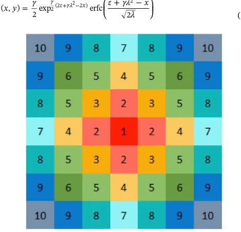
Seed movement by cultivation. Dispersal by cultivation is anisotropic with seeds being dispersed in the direction of travel (Lutman et al., 2002). In order to model the way in which seeds were moved by the combine, we assumed
⎜ ⎟ = ⎛ ⎝ + − ⎞ ⎠ + −
f x y γ ε γλ x
λ ( , )
2exp erfc 2
γ ε γλ x 2(2 2 )
2
2
(14) Table 1
Stages of theA. myosuroideslife-cycle identified as being affected by soil variability.
Life-cycle stage Soil property Effect Source
Germination Plant available water Total germination increases with hydrothermal time Colbach et al. (2006)and supplementary pot experiments
Germination Soil pH More seeds germinate at low pH Metcalfe et al. (2017) Pre-emergence herbicide mortality Soil organic matter Probability of survival increases with increasing soil
organic matter
Metcalfe et al. (2018a)
Seed production Soil organic matter Seed production increases with soil organic matter Supplementary pot experiments Seed production Water stress Seed production decreases when water is limiting Storkey and Cussans (2007)
This distribution matches the shape of that described by Paice et al. (1998)for anisotropic dispersal of seeds. The distribution is integrated for each grid cell in turn for a maximum of five grid cells in the di-rection opposite to the didi-rection of travel and then towards the direc-tion of travel until a total propordirec-tion of 0.999 is accounted for. Any remaining seeds are randomly allocated to a grid cell in the direction of travel, up to a maximum dispersal distance of 20 m. The direction of travel is set up along thexaxis of the grid from west to east for thefirst set of rows up to the width of the cultivator (40 m). It is then switched to travel east to west. The direction changes every time the number of rows reaches a multiple of the cultivator width.
For both natural dispersal and the seed movement by cultivation, if seeds are to be moved into a cell that lies outside of the model arena the process is reflected such that there is no immigration or emigration of seeds to and from thefield. This is representative of a realfield where boundaries are a source of seed (Marshall, 1989).
Vertical movement of seed in the soil. Seeds are moved vertically be-tween the shallow and deep soil layers. The tillage type can be set for each year to one of 4 types: plough, 20 cm tine, 10 cm tine, or < 5 cm tine. In years when the tillage is“plough”a proportion of seeds from the shallow soil layer are buried into the deep soil layer, conversely some seeds are brought up to the shallow soil layer. For all other tillage types there is no upward movement of seed (from the deep soil layer to the shallow soil layer) but a proportion of seeds are buried according to the depth of tillage.
3. Model parameterisation
Where possible, each function in the life-cycle model was para-meterised using data from the literature. However, the effect of soil organic matter (and its influence on water holding capacity) on A. myosuroides emergence and seed production was identified as a knowledge gap and so we set up an experiment under controlled con-ditions in order to parameterise these functions within the model (see supplementary material for experimental details).
3.1. A. myosuroides emergence
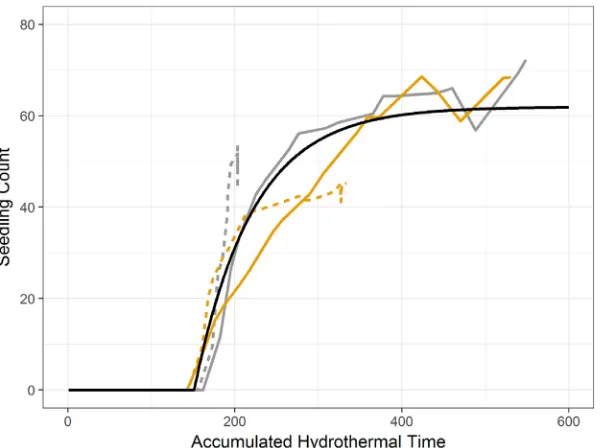
Colbach et al.'s parameterisation of Eq.(3)(2006, see supplemen-tary material) relies on information about the germinating seeds in-cluding the age and seed mass. To determine whether this para-meterisation works on soils with very different water holding capacities we germinated seeds of known origin, age and size on soil with different levels of organic matter (see supplementary material). The data from this experiment supported the shape of the Colbach curve but the offset parametertais increased to 49.169 in ourfit (Fig. 3). This offset in-creased the delay before the commencemenrt of germination to match the mean of our four treatments (Fig. 3).
Germination counts on different levels of soil pH collected by Metcalfe et al. (2017) show that the asymptote for germination is higher when soil pH is low. We therefore included a pH threshold of 6.5 in our model. At pH levels below this thresholdM(Eq.(3)) is increased by the ratio of the values for the asymptote of the curvesfitted to the low and high pH treatments respectively (40.92/36.72) (Metcalfe et al., 2017).
In the parameterisation of Eq.(3)(and Eqs. (18)–(26) in the sup-plementary materials) we set the age of the old cohort of seeds to 818 days and the new cohort to 60 days. Changing this parameter allowed the germination of seeds to occur at different rates. The mean Julian day of tillage,flowering ofA. myosuroidesand maturity ofA. myosur-oideswere set to be 258, 150, and 206 with respective variances 8, 3, and 6. These were determined usingfield data from a series offield experiments reported inStorkey and Cussans (2007)onA. myosuroides competition in winter wheat sown in the autumn and managed ac-cording to standard farm protocols except for the absence of herbicide. Depth was set to 1.5 cm and mean seed mass, determined by weighing
100 seeds, was 0.0014 g. Total available nitrogen was set at 25 kg/ha. FollowingColbach et al. (2002a,b), the base temperature (Tb) and water potentialψbforA. myosuroides(Eqs.(4)–(6)) were set at 0°C and
−1.53 MPa respectively.
3.2. Herbicide mortality
We modelled the survival rate ofA. myosuroidesafter the application of pre-emergence herbicides using data fromMetcalfe et al. (2018a). We took the data points for the proportion of seedlings surviving an application of pre-emergence herbicide at a dose equivalent tofield rate on different soils and plotted this against the organic matter (%) in the soil and fitted Eq. (9) to the data. The fitted values were η= 4.9,
ζ= 3.8252, andτ=−1.0890 (see supplementary Figure S.3). For post-emergence herbicide application we assume no effect of soil variability on contact herbicide efficacy and sopwasfixed at 0.3 (Bayer CropScience, 2017).
3.3. Seed production
Moss et al. (2010)parameterised their model of density dependent head production (Eq.(10)) with data from 16field experiments to give parameter valuesβ= 8.71 andα= 0.005741. We adjusted this equa-tion to account for soil organic matter according to the results from our experiment (see supplementary material). We only had one plant per pot, in our experiment, and so we would not expect this to be re-presentative of the number of heads produced underfield conditions but assumed the relative differences were representative of those seen underfield conditions. This allowed us to compute a generic ships between soil organic matter and the density dependent relation-ship between plants and heads (see supplementary material for deri-vation).
Parameters in Eq.(11)were derived forA. myosuroidesasϵ= 6.88 andρ=−4.61 from a series of glasshouse experiments reported in Storkey and Cussans (2007).
The mean (4.58) and standard deviation (0.23) of the lognormal distribution used to determine seed production per head are estimated from data provided by Moss (1990). The normal distribution:
(0.55, 0.126)is used to draw values for the proportion of viable seed, the mean and standard deviation are again estimated from the data provided byMoss (1990).
3.4. Seed losses
For the distributions used to calculate seed losses, data fromMoss (1990)were again used to estimate the means and standard deviations. The distributions used were: Log-normal(−0.81, 0.13) for above ground seed losses (e.g. through predation), and(0.3,0.077) for seed survival in the soil.
3.5. Seed movement
As was described byPaice et al. (1998), the mean (μ) of the natural dispersal distribution (Eq.(13)) is set at 0 and the standard deviation (σ) at 0.3. For seed movement by cultivation (Eq.(14)) parameters were set toγ= 10/3,λ= 0.1 andε=−0.15 to best match the shape of the distribution described byPaice et al. (1998)for anisotropic dispersal of seeds. The proportion of seeds moved vertically in the soil for each type of tillage was described byMoss (1990). Here stochasticity is added by drawing these from distributions estimated from the mean and range of that original data (Table 2)
4. Model validation
winter wheat. They sampled 136 locations in each field using an un-balanced nested sampling design, with pairs of points separated by
fixed distances. At each sampling point they counted the number ofA. myosuroidesseedlings emerging in the autumn. They also took soil cores to analytically determine the soil clay and silt content, soil organic matter, soil pH and soil gravimetric water content. The nested design structure allowed the partitioning of the components of variance for both A. myosuroides and soil properties at each of the spatial scales studied using the residual maximum likelihood (REML) estimator as described byMetcalfe et al. (2016), and scale-dependent correlations betweenA. myosuroidescounts and soil properties were calculated.
4.1. Patch location
To validate our model, we simulated three UK fields, for which complete datasets on soil properties and weed densities were available, studied byMetcalfe et al. (2018b). The threefields were Harpenden (Hertfordshire), Redbourn (Hertfordshire) and Haversham (Buck-inghamshire) (seeMetcalfe et al., 2018b). As an initial investigation, we kriged the measured soil data to predict on a 1-m grid. We then used this to parameterise the cells in the model. We simulated 40 years of weed growth starting with an initial seed bed of 10,000 seeds per cell, 20% of which were in the top soil layer. As we did not know the tillage history of the studiedfields, we simulated three typical tillage systems: (i) rotational cultivation with three years of tillage at < 5 cm followed by one year using the plough, (ii) tillage at 10 cm, and (iii) tillage at < 5 cm. We ran the model with all required input weather data on a daily timestep from Rothamsted met station (Hertfordshire, UK) be-ginning with data from 1966. We discarded the simulation results from
thefirst 10 years to allow the patches to stabilise following the initial seeding. We recorded and mapped the average number of plants si-mulated at each location in thefield (1 m × 1 m grid cell) across years 11–40 and for 10 different simulations of the model (a total of 300 realisations of thefield), we then compared these maps with the kriged distribution ofA. myosuroidesplants obtained byMetcalfe et al. (2018b) for thatfield.
4.2. Scale-dependent correlations
We wanted to see if the scale-dependent relationships betweenA. myosuroidesand soil properties found in thefield byMetcalfe et al. (2018b)were an emergent property of the model. To do this we needed to simulate soil realistic of that found in thefields, but that maintained
fine-scale variation, which is lost in the kriged maps. We simulated soil properties on a 1 m × 1 m grid using lower upper decomposition of the covariance matrix, also known as the Cholesky decomposition tech-nique (Webster and Oliver, 2007, chapter 12). We created the covar-iance matrix for each soil property in eachfield from the covariance function corresponding to the spherical variogramfitted to the soil data and conditioned the simulation to include our measured soil properties at the location where they were measured. TheRconditioning data were transformed to standard normal form (denoted by the vectorz) and the values atSunsampled positions were drawn independently at random from a standard normal distribution (vectorg). To obtain the vector of conditionally simulated values (y) we used
= ⎡ ⎣
⎢ − + ⎤⎦⎥
y
z
L L L g
R
S
SR SS1 RR (15)
whereLis the lower triangular matrix obtained from the decomposition of the covariance matrix for thefield.
Following the simulation of the soil, we scaled the simulated values to match the mean and range of the original data values:
= − × +
y x m
s sobs mobs (16)
wherexis a simulated value,mandsare the mean and standard de-viation respectively of all the simulated values for that soil property and mobsandsobsare the mean and standard deviation respectively for the observed data. Ideally we would have simulated all soil properties based on their covariances. However, due to the size of thefield and the spatial scale of simulation this was not possible and so we performed a Fig. 3.Germination counts plotted against hydrothermal time. Grey is low soil organic matter, Yellow is medium soil organic matter. Solid lines show high water input and dashed lines are low water input. The solid black line shows the resulting germination counts from Eq.(3)when parameterised for the seeds used in the experiment. See supplementary material for experimental detail.
Table 2
Distributions used to sample the proportion of seeds to be moved between soil layers due to tillage.
Tillage type Direction of movement Distribution type Mean Variance
Plough Shallow to deep Lognormal −0.0515 0.0191 Deep to shallow Lognormal −1.0670 0.1199 20 cm tine Shallow to deep Normal 0.2000 0.0510
Deep to shallow None
10 cm tine Shallow to deep Normal 0.4000 0.1010 Deep to shallow None
number of checks to prevent the simulation of impossible soil dis-tributions. We checked that the scaled simulated values did not exceed realistic ranges for these soil properties and discarded any simulations falling outside of the acceptable range. We also checked that the si-mulated clay and silt values did not sum to values greater than 100 and so we paired simulations accordingly. We produced 35 suitable simu-lations for each soil property for the Harpenden and Havershamfields (the Redbournfield was too large to simulate in this way).
We simulated 40 years of weed growth starting with an initial seed bed of 10,000 seeds per cell, 20% of which were in the top soil layer. We implemented 10 cm tine as the tillage type. We ran the model with weather data from Rothamsted met station (Hertfordshire, UK) begin-ning with data from 1966.
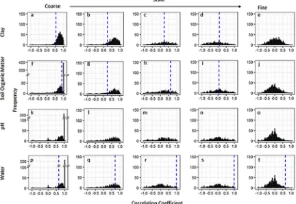
We took the output of the model only for years 11–40 from each simulation and extracted the number of simulatedA. myosuroidesplants at each of the sampling locations from the original study (Metcalfe et al., 2018b). We did the same analysis of the nested sampling design as described by Metcalfe et al. (2016)to give scale-dependent corre-lation coefficients between the simulated A. myosuroidescounts and each soil property present in the model (clay, organic matter, pH and water) for each of the 1050 realisations of thefield. We plotted a his-togram to look at the frequency of these correlations across all 1050 realisations of the field given by the model and compared this dis-tribution to the value obtained in thefield data for each spatial scale and each soil property (Metcalfe et al., 2018b).
5. Results
5.1. Patch location
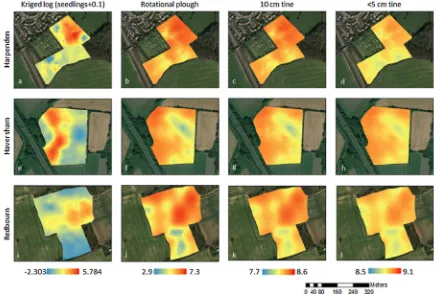
The locations of the patches predicted by the model were broadly
similar to those observed in thefield study (Fig. 4). At a coarse scale there are broad similarities between the distribution ofA. myosuroides observed in thefield and the predicted distributions from the model for allfields. In Harpenden, the rotational ploughing system led to very similar distributions, whereas the other two tillage systems (10 cm tine, and < 5 cm tine) showed much more uniform distributions across the
field (Fig. 4a–d). For thefield in Redbourn theA. myosuroidescounts in the eastern part of thefield were reflected in the predictions, as were the low counts in the southern part of thefield. However, in the west the observed and predicted distributions differ (Fig. 4i–l). Finally, in Haversham the western part of thefield shows similar patch locations to those observed in thefield (Fig. 4e–h). In all cases the predicted seedling densities are larger than were observed in thefield and the patches more extensive.
5.2. Scale-dependent correlations
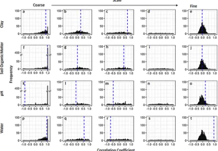
The scale-dependent correlations betweenA. myosuroidesand clay were fairly consistent with those observed in thefield. At coarse scales the model simulations largely resulted in large positive correlations (Figs. 5a and6a). For Harpenden, this was close to the observed cor-relation in thefield of 0.85 and for Haversham the simulated correla-tions were often larger than that observed in thefield (0.55), whereas at intermediate scales (Figs. 5b–d and6b–d) where the observed corre-lation in thefield were weaker the prediction from the models were less conclusive with a range of correlation coefficients that included both positive and negative values. At thefinest scale all correlations between clay content and the simulatedA. myosuroidesseedling densities were small and often close to zero. This reflects the non-significant correla-tions observed in Harpenden and Havershamfields.
The results were similar for the relationships predicted between soil
organic matter and A. myosuroidesseedling densities with the model predicting large positive relationships with organic matter at coarse scales (Figs. 5f and6f). There was no distinct pattern in the correlation coefficients at intermediate scales in Harpenden (Fig. 5g–i) and only small positive correlations at intermediate scales in Haversham (Fig. 6g and h), which were similar to the observed correlations of 0.22 and 0.62 at those scales. In bothfields there were correlation coefficients close to zero at the finest scale between soil organic matter and A. myosuroides(Figs. 5j and6j).
When we consider pH and its relationship with A. myosuroides seedling densities in the Harpendenfield wefind a large peak of posi-tive correlation coefficients at coarse scales (Fig. 5k), which is in con-trast to the negative correlation coefficient observed int hefield. Again, at intermediate scales (Fig. 5l–n) there is no distinct pattern in the correlation coefficients and atfine scales all correlation coefficients are close to zero. In Haversham the REML model used to partition the variance across scales could not be fitted to thefield data and so no comparison can be made with the simulated model outputs.
We found positive relationships with soil moisture content at the coarse-scale in the majority of simulations (Figs. 5p and6p). This result matched the significant positive correlation we found in thefields at this spatial scale. At intermediate scales (Figs. 5q–s and 6q–s), the correlations between soil water content andA. myosuroides densities predicted by the model were less consistent. At thefinest scale (Figs. 5t and6t) the relationship between soil water content andA. myosuroides seedling counts predicted by the model was often close to zero in both
fields. However, at thisfine scale ourfield observations gave quite large correlations and lay outside of the distribution of correlations predicted by our model.
6. Discussion
Our results support in-field studies (Lutman et al., 2002; Murdoch et al., 2014; Metcalfe et al., 2018b) that show soil is an important de-terminant in the within-field distribution ofA. myosuroides. Our results suggest that our model can provide a good prediction of the location of patches withinfields. Irrespective of the tillage type implemented in the model the spatial distribution ofA. myosuroidesseedlings across 300 realisations was consistent with observedfield distributions (Fig. 4). This indicates the usefulness of this model in locatingA. myosuroides vulnerable zones withinfields.
Simulated seedling densities were quite different under the different tillage types, yet all provided a good estimation of patch location. This supports the conclusions fromColbach et al. (2000)that densities are often highly variable and so the prediction of densities is less accurate than the prediction of patch location. This means that it is possible to predict patch locations or weed vulnerable zones irrespective of the tillage practices in place on a farm, making the model useful as a de-cision support tool as it is not necessary to provide all the information about cultivation history in order to locate weed vulnerable zones. Our model was built to answer the question of the impact of soil variation on the distribution of the weed and so relative abundances are a useful output, and absolute values are not particularly important.
existing or supplemented soil maps, already in use on farm for other site-specific management practices, then we should be able to predict the likelihood of parts of thefield being vulnerable toA. myosuroides and so be able to develop maps for patch spraying based on the output of this model.
As with all models of weed population dynamics there are some limitations to this model including a lack offield data, and the adoption of number of assumptions. However these are necessary in order to keep the model simple enough to be functional whilst retaining enough detail to understand the system (Fernandez-Quintanilla, 1988). Initially some of the limitations of the model come due to a lack offield data and are also under-represented in other models of A. myosuroidessuch as those byMoss (1990)andColbach et al. (2006). These include the fate of seeds after shedding, where we have included a certain amount of seed loss but this is an all encompassingfigure, including predation and decay, which would be difficult to model mechanistically. Similarly for other life-cycle processes where we only have information on the range and mean offield data such as seed production. In these cases we draw values stochastically but the chosen values remain unaffected by other processes within the life-cycle. In our model we assume that the density of the crop and other weeds are uniform across thefield and so spatial variability in interspecific competition is excluded. As we base this model on the premise that thefield is a heterogeneous environment this may not be a correct assumption to make, however, it is an assumption that is also made in other models for patch spraying purposes (e.g.Paice et al., 1998). In this regard, our model could be improved by modelling interspecific competition mechanistically. In order to simplify the model we have divided the soil into two layers: a shallow layer from which seeds can germinate and a deep layer. However, in reality the soil is a continuum and there will be a gradient over which seeds can
germinate at different rates. Finally, natural seed dispersal is bar-ochorous in our model and seeds are moved by the combine and cul-tivator. Both of these methods of dispersal are independent of other factors, yet it has been shown that there can be some influence of wind speed on seed dispersal ofA. myosuroides(Colbach and Sache, 2001) and equally, seed movement in the soil can depend on soil properties (Benvenuti, 2007).
In our model validation, the large scale correlations betweenA. myosuroidesand soil properties were generally similar to those observed in the field. However, for soil pH our simulations predicted positive correlations at large scales, whereas the observed data showed a ne-gative correlation. The only role of soil pH in our model is in altering the asymptote reached in germination. We implemented this using a threshold approach, where the asymptote for germination is increased when soil pH is below 6.5. It is possible that this is insufficient to de-scribe the true nature of the impact of soil pH on germination as by only changing the asymptote we will only see these differences in years when there are very large numbers of seeds germinating. It is likely that the observed response to pH in thefield data is a product of additional processes to do with growth and competition in the established phase that are not currently captured in the model.
the appropriate scale.
7. Conclusions
We have drawn together experimental data on the impact of soil properties on the life-cycle and management of this important agri-cultural species and through a modelling approach demonstrated the important role played by soil properties in determining the within-field distribution of A. myosuroides. We have also shown that scale-depen-dent correlations betweenA. myosuroidesand soil properties observed in thefield are an emergent property of this model, which incorporates small changes to individual components of the life-cycle due to soil properties. This could allow it to become an effective management tool as the coarse-scale correlations, which are shown to be of the greatest importance, are the ones that have the most relevance to management.
Acknowledgements
Rothamsted Research receives grant aided support from the Biotechnology and Biological Sciences Research Council (BBSRC) of the United Kingdom. This research was funded by the Natural Environment Research Council (NERC) and the Biotechnology and Biological Sciences Research Council (BBSRC) under research programme NE/ N018125/1 LTS-M ASSIST Achieving Sustainable Agricultural Systems. The project was funded by a BBSRC Doctoral Training Partnership in Food Security BB/J014451/1 and the Lawes Agricultural Trust. We thank the Lawes Agricultural Trust and Rothamsted Research for weather data from the e-RA database.
Appendix A. Supplementary data
Supplementary data associated with this article can be found, in the online version, athttps://doi.org/10.1016/j.ecolmodel.2018.11.002.
References
Allen, R.G., Pereira, L.S., Raes, D., Smith, M., 1998. Crop Evapotranspiration–Guidelines for Computing Crop Water Requirements–FAO Irrigation and Drainage Paper 56. FAO, Rome 300 (9).
Bayer CropScience, 2017. Atlantis WG–Don’t wait until March. Available at:http:// cropscience.bayer.co.uk/our-products/herbicides/atlantis-wg/dont-wait-until-march/[Accessed 17 August 2017].
Benvenuti, S., 2007. Natural weed seed burial: effect of soil texture, rain and seed characteristics. Seed Sci. Res. 17 (3), 211–219.
Castaldi, F., Pelosi, F., Pascucci, S., Casa, R., 2016. Assessing the potential of images from unmanned aerial vehicles (UAV) to support herbicide patch spraying in maize. Precis. Agric. 18 (1), 76–94.
Christensen, S., Søgaard, H.T., Kudsk, P., Norremark, M., Lund, I., Nadimi, E.S., Jorgensen, R., 2009. Site-specific weed control technologies. Weed Res. 49, 233–241. Colbach, N., Forcella, F., Johnson, G.A., 2000. Spatial and temporal stability of weed
populations overfive years. Weed Sci. 48 (3), 366–377.
Colbach, N., Sache, I., 2001. Blackgrass (Alopecurus myosuroidesHuds.) seed dispersal from a single plant and its consequences on weed infestation. Ecol. Model. 139 (2), 201–219.
Colbach, N., Chauvel, B., Dürr, C., Richard, G., 2002a. Effect of environmental conditions onAlopecurus myosuroidesgermination. I. Effect of temperature and light. Weed Res. 42 (3), 210–221.
Colbach, N., Dürr, C., Chauvel, B., Richard, G., 2002b. Effect of environmental conditions onAlopecurus myosuroidesgermination. II. Effect of moisture conditions and storage length. Weed Res. 42 (3), 222–230.
Colbach, N., Dürr, C., Roger-Estrade, J., Chauvel, B., Caneill, J., 2006. AlomySys: Modelling black-grass (Alopecurus myosuroidesHuds.) germination and emergence, in interaction with seed characteristics, tillage and soil climate: I. Construction. Eur. J. Agron. 24 (2), 95–112.
Colbach, N., Chauvel, B., Gauvrit, C., Munier-Jolain, N.M., 2007. Construction and eva-luation of ALOMYSYS modelling the effects of cropping systems on the blackgrass life-cycle: from seedling to seed production. Ecol. Model. 201 (3), 283–300. Department for Environment, Food & Rural Affairs (Defra), 2013. Farm Practices Survey
Autumn 2012–England.
Dieleman, J.A., Mortensen, D.A., Buhler, D.D., Cambardella, C.A., Moorman, T.B., 2000. Identifying associations among site properties and weed species abundance. I. Multivariate analysis. Weed Sci. 48 (5), 567–575.
Dunker, M., Nordmeyer, H., Richter, O., 2002. Modellierung der Ausbreitungsdynamik vonAlopecurus myosuroidesHuds. Für eine teilflächenspezifische
Unkrautbekämpfung. Z. Pflanzenkrankh. Pflanzenschutz Sonderh. 18, 359–366.
Fernandez-Quintanilla, C., 1988. Studying the population dynamics of weeds. Weed Res. 28 (6), 443–447.
Frank, E.C., Lee, R., 1966. Potential solar beam irradiation on slopes, U.S. Forest Service Research Paper RM-18.
Frere, M., Popov, G.F., 1979. Agrometeorological Crop Monitoring and Forecasting. FAO. Garibay, S.V., Richner, W., Stamp, P., Nakamoto, T., Yamagishi, J., Abivardi, C., Edwards, P.J., 2001. Extent and implications of weed spatial variability in arable cropfields. Plant Prod. Sci. 4 (4), 259–269.
Gebbers, R., Adamchuk, V.I., 2010. Precision agriculture and food security. Science 327, 828–831.
Gonzalez-Andujar, J.L., Perry, J.N., Moss, S.R., 1999. Modelling effects of spatial patterns on the seed bank dynamics ofAlopecurus myosuroides. Weed Sci. 47 (6), 697–705. Grundy, A.C., 2003. Predicting weed emergence: a review of approaches and future
challenges. Weed Res. 43 (1), 1–11.
Hollis, J.M., Hannam, J., Bellamy, P.H., 2012. Empirically-derived pedotransfer functions for predicting bulk density in European soils. Eur. J. Soil Sci. 63 (1), 96–109. Holm, L.G., Doll, J., Holm, E., Pancho, J., Herberger, J., 1997. World Weeds: Natural
Histories and Distribution. John Wiley & Sons, New York, USA.
Holst, N., Rasmussen, I.A., Bastiaans, L., 2007. Field weed population dynamics: a review of model approaches and applications. Weed Res. 47 (1), 1–14.
Howard, C.L., Mortimer, A.M., Gould, P., Putwain, P.D., Cousens, R., Cussans, G.W., 1991. The dispersal of weeds: seed movement in arable agriculture. Brighton Crop Protection Conference–Weeds, vol. 2 821–828.
Krohmann, P., Gerhards, R., Kühbauch, W., 2006. Spatial and temporal definition of weed patches using quantitative image analysis. J. Agron. Crop Sci. 192 (1), 72–78. Kropff, M.J., 1993. Mechanisms of competition for light. Modelling Crop-Weed
Interactions. pp. 33–61.
Kropff, M.J., van Kraalingen, D.W.G., van Laar, H.H., 1993. Program Structure of the Model INTERCOM.
López-Granados, F., Torres-Sánchez, J., De Castro, A.I., Serrano-Pérez, A., Mesas-Carrascosa, F.J., Peña, J.M., 2016a. Object-based early monitoring of a grass weed in a grass crop using high resolution UAV imagery. Agron. Sustain. Dev. 36 (4), 67. López-Granados, F., Torres-Sánchez, J., Serrano-Pérez, A., de Castro, A.I.,
Mesas-Carrascosa, F.J., Peña, J.M., 2016b. Early season weed mapping in sunflower using UAV technology: variability of herbicide treatment maps against weed thresholds. Precis. Agric. 17 (2), 183–199.
Lutman, P.J.W., Perry, N.H., Hull, R.I.C., Miller, P.C.H., Wheeler, H.C., Hale, R.O., 2002. Developing a Weed Patch Spraying System for Use in Arable Crops. Home Grown Cereals Authority, London.
Maréchal, P.Y., Henriet, F., Vancutsem, F., Bodson, B., 2012. Ecological review of black-grass (Alopecurus myosuroidesHuds.) propagation abilities in relationship with her-bicide resistance. Biotechnol. Agron. Soc. Environ. 16 (1), 103.
Marshall, E.J.P., 1989. Distribution patterns of plants associated with arablefield edges. J. Appl. Ecol. 26 (1), 247–257.
Metcalfe, H., Milne, A.E., Webster, R., Lark, R.M., Murdoch, A.J., Storkey, J., 2016. Designing a sampling scheme to reveal correlations between weeds and soil prop-erties at multiple spatial scales. Weed Res. 56 (1), 1–13.
Metcalfe, H., Milne, A.E., Murdoch, A.J., Storkey, J., 2017. Does variable soil pH have an effect on the within-field distribution ofA. myosuroides? Asp. Appl. Biol. 134, 145–150.
Metcalfe, H., Milne, A.E., Hull, R., Murdoch, A.J., Storkey, J., 2018a. The implications of spatially variable preemergence herbicide efficacy for weed management). Pest Manage. Sci. 74 (3), 755–765.
Metcalfe, H., Milne, A.E., Webster, R., Lark, R.M., Murdoch, A.J., Kanelo, L., Storkey, J., 2018b. Defining the habitat niche of black-grass (Alopecurus myosuroides) at thefield scale. Weed Res. 52 (3), 165–176.
Moss, S.R., 1980. The agro-ecology and control of black-grass,Alopecurus myosuroides Huds., in modern cereal growing systems. ADAS Quart. Rev. 38, 170–191. Moss, S.R., 1990. The seed cycle ofAlopecurus myosuroidesin winter cereals: a
quanti-tative analysis. In: EWRS (European Weed Research Society) Symposium. Helsinki, Finland.
Moss, S.R., Tatnell, L.V., Hull, R., Clarke, J.H., Wynn, S., Marshall, R., 2010. Integrated management of herbicide resistance, HGCA Project Report 466.
Murdoch, A.J., Pilgrim, R.A., de la Warr, P.N., 2010. Proof of concept of automated mapping of weeds in arablefields, HGCA Project Report. pp. 471.
Murdoch, A.J., Flint, C., Pilgrim, R.A., de la Warr, P.N., Camp, J., Knight, B., Lutman, P., Magri, B., Miller, P., Robinson, T., Sandford, S., Walters, N., 2014. Eyeweed: auto-mating mapping of black-grass (Alopecurus myosuroides) for more precise applications of pre- and post-emergence herbicides and detecting potential herbicide resistance. Asp. Appl. Biol.–Crop Production in Southern Britain: Precision Decisions for Profitable Cropping 127, 151–158 Association of Applied Biologists, Wellesbourne, UK.
Osakabe, Y., Osakabe, K., Shinozaki, K., Tran, L.S.P., 2014. Response of plants to water stress. Front. Plant Sci. 5, 86.
Paice, M.E.R., Day, W., Rew, L.J., Howard, A., 1998. A stochastic simulation model for evaluating the concept of patch spraying. Weed Res. 38, 373–388.
Pederson, H.J., Kudsk, P., Helwig, A., 1995. Adsorption and ED 50 values offive soil-applied herbicides. Pestic. Sci. 44, 131–136.
Penman, H.L., 1948. Natural evaporation from open water, bare soil and grass. Proc. R. Soc. Lond. A: Math. Phys. Eng. Sci. 193 (1032), 120–145.
Penman, H.L., 1956. Estimating evaporation. EOS Trans. Am. Geophys. Union 37 (1), 43–50.
Penman, H.L., 1963. Vegetation and hydrology. Soil Sci. 96 (5), 357.
Rew, L.J., Cousens, R.D., 2001. Spatial distribution of weeds in arable crops: are current sampling and analytical methods appropriate? Weed Res. 41 (1), 1–18.
Storkey, J., Cussans, J.W., 2000. Relationship between temperature and the early growth ofTriticum aestivumand three weed species. Weed Sci. 48 (4), 467–473. Storkey, J., Cussans, J.W., 2007. Reconciling the conservation of in-field biodiversity with
crop production using a simulation model of weed growth and competition. Agric. Ecosyst. Environ. 122 (2), 173–182.
Stratonovitch, P., Storkey, J., Semenov, M.A., 2012. A process-based approach to mod-elling impacts of climate change on the damage niche of an agricultural weed. Global Change Biol. 18, 2071–2080.
Tian, L.F., Steward, B.L., Tang, L., 2000. Smart sprayer project: sensor-based selective herbicide application system. Environ. Ind. Sens. 73–80.
van Genuchten, M.T., 1980. A closed-form equation for predicting the hydraulic con-ductivity of unsaturated soils. Soil Sci. Soc. Am. J. 44 (5), 892–898.
Webster, R., Oliver, M.A., 2007. Geostatistics for Environmental Scientists, 2nd ed. John Wiley & Sons, Chichester.
Wilson, B.J., Brain, P., 1991. Long-term stability of distribution ofAlopecurus myosuroides Huds. within cerealfields. Weed Res. 31 (6), 367–373.