Static Conversion of a Salinity Difference into a
Temperature Difference: A Heat and Mass Transfer
Investigation
Matteo Morciano, Matteo Fasano, Pietro Asinari * and Eliodoro Chiavazzo *
Department of Energy, Politecnico di Torino, Corso Duca degli Abruzzi 24, Torino 10129, Italy; [email protected] (M.M.); [email protected] (M.F.)
* Correspondence: [email protected] (P.A.); [email protected] (E.C.); Tel. +39-011-090-4434 (P.A.); +39-011-090-4557 (E.C.).
Abstract: In this work, we experimentally investigate mass and heat transport phenomena in a modular device while converting a solution salinity difference into a temperature difference. Operations occur under fixed total ambient pressure and without mechanical moving parts, thus realizing a fully static conversion. Provided that a constant salinity gradient can be imposed, the proposed device is able to generate a steady cooling capacity. Here, we purposely operate with environmentally benign and easily accessible sodium chloride water solutions only. A numerical model is finally elaborated, validated and used to explore a wider range of possible device configurations and operating conditions.
Keywords:condensed matter; heat transfer; mass transfer; thermodynamics
1. Introduction
We investigate heat and mass transport phenomena occurring in a fully static (i.e. with no moving mechanical parts) cooling device, which has been experimentally tested and interpreted by a simplified one-dimensional theoretical model. The realized lab-scale prototype operates at ambient pressure and consists of several identical stages, which are designed to generate a cooling capacity inducing multiple evaporation/condensation processes. Such processes are driven by a salinity difference between two water solutions, which can be separated for instance by a hydrophobic membrane [1–3]. Here, we present both the preliminary experimental results and predictions by the numerical model. The latter is only intended to reasonably extrapolate the expected behavior of the device under a wider range of operating conditions. More specifically, we estimate the cooling performance at different salinity values of the solutions, thermal loads, number of stages, and other relevant geometrical quantities of our design. It is interesting noticing that, in the proposed set-up, the constant salinity difference needed for sustaining the cooling load may be possibly maintained using passive solar regeneration as discussed by the Authors of this work in a previous study [4], thus paving the way to a static cooling cycle driven by solar power.
2. Materials and methods
2.1. Schematic and working principle
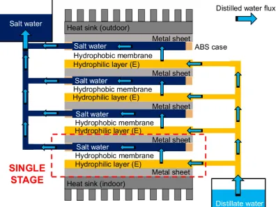
low thermal resistance. Here, aluminum plates with size 13×13 cm2are used between the stages. Relaying upon capillarity, a thin hydrophilic stripe is connected to the hydrophilic layer located at the bottom of each stage and ensures a continuous supply of distilled water from a storage basin without the need of a pump or any other circulation means.
In Figure1, the hydrophilic layer is labeled with (E), which stands for evaporator. On the other hand, the saltwater basin is located at the top: such a configuration possibly ensures a favorable salinity stratification.
The difference in salinity (and in water activity) causes a vapor pressure disparity between the two condensed phases, which is in turn responsible for a net water vapor flux from the hydrophilic layer towards the NaCl solution. Hence, the former acts as an evaporator, whilst the latter as a condenser. A latent heat transfer therefore occurs in this process, and this establishes a temperature difference across the membrane. As a result the saltwater is heated up, while the distilled water in the hydrophilic layers is cooled down.
Figure 1.Schematic of the considered lab-scale cooling device (4-stages).
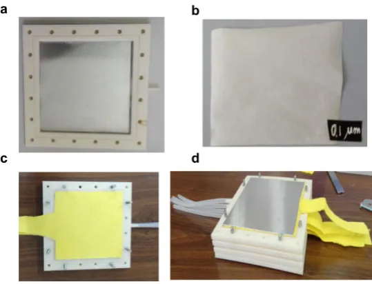
In Figure2, the main components of our specific realization are shown. In detail, we report pictures of the cavity where saltwater is accommodated (i.e. condenser,≈6 mm thickness), the hydrophobic microporous membrane (polytetrafluoroethylene, with pore size 0.1µm and thickness≈0.15 mm),
Figure 2. Main components of the tested lab-scale prototype. (a) Cavity for the saltwater (i.e. condenser). (b) Microporous membrane with pore size 0.1µm. (c) Hydrophilic layer wet by distillate
(i.e. evaporator). (d) Assembled lab-scale cooling device (4-stages).
To assess the performances of the cooling device, we adopted the experimental setup depicted in Figure3. The setup includes a laptop, a data acquisition (DAQ) board (National Instruments), a digital refractometer, a scale (balance), the designed lab-scale prototype and a thermal user. The data acquisition board collects four temperature measures by thermocouples, namely the temperature drop across the prototype, the outdoor and the indoor (inside the thermal user) temperatures. The scale is used to assess the mass change in the saltwater basin due to the distilled water flow through the membranes. A digital refractometer is finally used to monitor the salinity in the saltwater and distillate basins.
Figure 3.Experimental setup for testing the performances of the cooling device.
experimentally assessed asTRuser ≈ 0.9±0.15WK−1. In Figure4, the intersection between curves
represents the equilibrium operating condition: in the considered setup, the obtained temperature difference between wooden box and ambient temperature is≈1◦C, with a cooling capacity of≈1.12 W.
0 2 4 6 8
−8 −6 −4 −2 0
Power [W]
Indoor temperature drop [°C]
Cooling capacity
User demand
N = 4, Y = 170, T
out = 26°C
TRuser≈ 0.9 W K−1
Figure 4.Operating condition at equilibrium: intersection between cooling capacity (N =4 stages) and user demand curves.
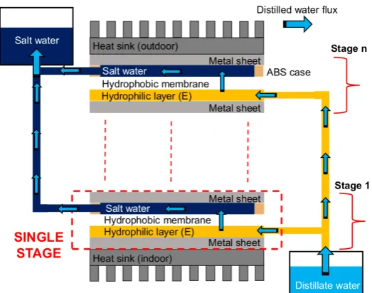
We notice that our cooling device is highly modular: depending on the target in terms of cooling capacity, a variable amount of stages could be easily assembled (see Figure5), as well as different salinity could be adopted (below the saturation limit at the operating temperature).
Figure 5.Schematics of an−stages version of the proposed cooling device.
2.2. Theoretical background
Mass transfer
The driving force of the cooling effect is the salinity gradient that, in each stage, induces a temperature drop between evaporator and condenser of each stage [2,3]. In fact, this salinity gradient creates a vapor pressure difference across the membrane:
∆pw =a(YE)pw(TE)−a(YC)pw(TC), (1)
whereadenotes the water activity;YEandYCare the mass fractions of salt (Y =msalt/msolution) at
the evaporator (distilled water) and at the condenser (saltwater), respectively; TE andTC are the
temperatures of distilled and saltwater, respectively.
Raoult’s law can be used to approximately (i.e. under the assumption of ideal mixture) compute the activity of the NaCl/water solution:
a= MNaCl(1−Y)
MNaCl+NionMH2OY−MNaClY
, (2)
where Nion = 2 for NaCl, while MNaCl andMH2Oare the molar masses (expressed in [g/mol]) of
sodium chloride and water, respectively. The considered water/NaCl solution has a salinity of 170 g/l (YE =0.170); therefore, equation2predictsa(YE)≈0.888. On the other side, the activity of distilled
water is clearlya(YC) =1.
The vapor pressure can be instead computed via the Antoine’s semi-empirical correlation:
logpw=A− B
C+T, (3)
whereA, BandCare the component-specific constants, which in this case are estimated as 8.07, 1730.63 and 233.42, respectively.
The specific mass flow rate (J,[kg/s/m2]) through the membrane is proportional to the partial pressure gradient (∆pw) and the characteristic permeability coefficient (K), namely
J=K∆pw. (4)
In this study, the permeability coefficient is approximately estimated as:
K=
1 eDMH2O
RTdmem
+ DM1
H2O RTdgap air
−1
, (5)
whereeis the porosity of membrane,D[m2/s]is the vapor diffusion coefficient in air (≈ 0.282×
10−4[m2/s]) at the mean stage temperatureT,Ris the gas constant (8.314[J/K/mol]),d
mem is the
membrane thickness, while dgap air represents an effective air gap thickness taking into account
non-ideal contact between the membrane and the hydrophilic layer. Actually,dgap airis a fine-tuned
parameter to match experimental results. We stress that equation (5) only includes the Fickian diffusion regime. This is clearly an approximation as, for instance, the Knudsen transport regime is neglected.
Heat transfer
The net heat flux (Q) between the hydrophilic layer and the saltwater cavity is given by a balance between the water phase change and the conduction heat transfer through the stages:
Q=J∆Hv−
ke f f,gap
dgap
(TC−TE), (6)
whereke f f,gapis the effective thermal conductivity of the gap (including heat conduction through air
and membrane), whereas∆Hvis the latent heat of water vaporization (2272 [kJ/kg]).
The thermal resistance of the saltwater cavity in each stage was estimated assuming natural convection. In particular, we considered the Nusselt-Rayleigh correlation from [5]. To this end, we compute the Rayleigh number as:
Ra= gβh
3(T
E−TC)
να , (7)
whereg[ms−2]is the acceleration of gravity,βis the thermal expansion coefficient of water (207×
10−6[K−1]at ambient temperature),his the thickness of saltwater cavity (≈6 mm),αis the thermal
diffusivity of water (0.143×10⁻⁶[m2s−1]) andνis the kinematic viscosity of water (1×10⁻⁶[m2s−1]).
Hence, based on empirical correlations reported in literature, we estimated the Nusselt number as Nu
≈1.58 [5].
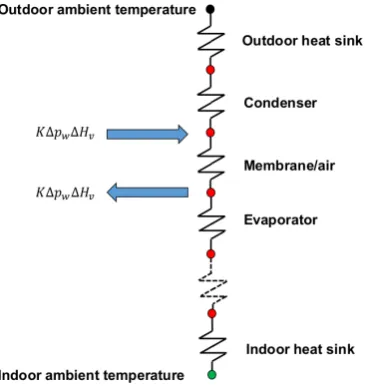
For the sake of completeness, in Figure6, a schematic representation of the numerical model is reported in terms of an equivalent thermal resistance circuit.
Figure 6. Equivalent thermal resistance circuit schematically representing the one-dimensional theoretical model.
3. Results
3.1. Experimental performances
Experimental results are obtained by testing the 4-stages device presented in Figures2and3, where a water solution with salinity of 170 g/l is considered. During the experiments, the ambient temperature was maintained approximately constant at 26±0.3◦C.
drop across the four stages of our cooling device was≈2◦C; whilst the temperature drop between ambient and thermal user was 1.2±0.25◦C.
Hence, considering the aforementioned overall thermal transmittance of the wooden box (≈
0.9±0.15WK−1), the cooling capacity was estimated≈77±20Wm-2, with an average specific flux of distilled water equal to≈1658±129[gm-2h-1]. Concurrently, the mass flux was obtained by measuring the mass change over time in the saltwater basin (sampling period: 15 minutes).
In addition, we also measured the maximum cooling capacity corresponding to a vanishing temperature difference across the entire device (hence between the ambient and the thermal user, too). In this test, an electrical resistance was attached to the heat sink in the wooden box (thermal user) thus providing the necessary thermal power to impose a steady∆T = 0 across the cooling device. Under the above conditions, we measured≈103±4Wm-2cooling capacity, with an average specific mass flux towards the saltwater basin of≈1837±251[gm-2h-1]. Those two experimental operating conditions are reported by red circles in the figures of this manuscript and are the minimum set of data to infer the (almost linear) characteristic cooling curve of our device in a typical chart reporting the cooling power versus the temperature drop.
3.2. Modeling results
Theoretical performances of the cooling device obtained by the equations described in Section 2.2were also investigated. A wide range of possible configurations is explored. In particular, the following parameters have been considered and varied:
• Number of stages (N);
• Thickness of air gap between the hydrophobic membrane and the hydrophilic layer (δ); • Salinity of the water/NaCl solution (Y);
• Outdoor ambient temperature (Tout).
Effect of number of cooling stages
The estimated cooling capacity and the specific mass flow rate of the distilled water are plotted in Figure7as function of the number of cooling stages and indoor temperature drop. In this study, we specifically consider the performances of 1,2,3,4 and 10-stages setups.
0 20 40 60 80 100 120
−8 −6 −4 −2 0
Cooling capacity [W m−2]
Indoor temperature drop [°C]
Mod. results N = 1 Mod. results N = 2 Mod. results N = 3 Mod. results N = 4 Mod. results N = 10 Exp. results N = 4 Y = 170, T
out = 26°C,
δ = 0.1 mm
0 1 2 3 4 5
−8 −6 −4 −2 0
Mass flow rate [l h−1 m−2]
Indoor temperature drop [°C]
Y = 170, T
out = 26°C,
δ = 0.1 mm
Figure 7.Experimental and modeling performances of the cooling device prototyped with varying number of operating stages. (Left) Cooling capacity and (Right) specific mass flow rate are depicted. Modeling predictions are represented by colored lines, whereas experimental measures by red circles.
Effect of air gap thickness
An air gap can be added between the hydrophobic membrane and the hydrophilic layer in each cooling stage, in order to increase the local thermal resistance. Such gap can be imposed by introducing a rigid spacer with large porosity between the membrane and the evaporator. In this case, the thickness of the air gap (δ) becomes a significant design parameter of the cooling device, and it is worth to be
investigated by sensitivity analysis. Different air gap thicknesses are evaluated, and the results plotted in Figure8. In particular, we have consideredδ=0.05, 0.1, 0.5 mm.
0 20 40 60 80 100 120
−8 −6 −4 −2 0
Cooling capacity [W m−2]
Indoor temperature drop [°C]
Mod. results δ = 0.05 mm Mod. results δ = 0.1 mm Mod. resutls δ = 0.5 mm Exp. results δ = 0.1 mm
N = 4, Y = 170, T
out = 26°C
0 0.5 1 1.5 2 2.5
−8 −6 −4 −2 0
Mass flow rate [l h−1 m−2]
Indoor temperature drop [°C]
N = 4, Y = 170, T
out = 26°C
Figure 8.Experimental and modeling performances of the cooling device prototyped with varying air gap thicknessδ. (Left) Cooling capacity and (Right) specific mass flow rate are depicted. Modeling
predictions are represented by colored lines, whereas experimental measures by red circles.
Results show that a larger air gap thickness can lead to reduced distilled water needs (and cooling capacity). For example, an increase from δ = 0.1 mm to δ = 0.5 mm induces a≈ 110% specific
mass flow rate drop, with a≈15% cooling capacity reduction at the same time (at zero temperature difference between ambient and thermal user).
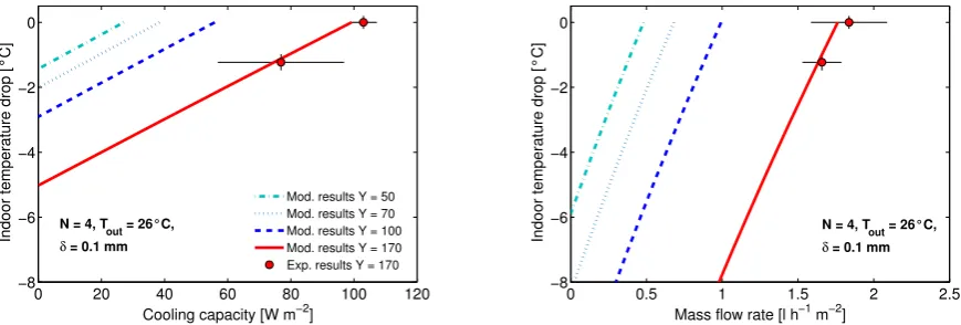
Effect of salinity
Four different salt concentrations are then considered. In particular, 50, 70, 100, 170 g/l are considered in our simulations, with results shown in Figure9.
0 20 40 60 80 100 120 −8
−6 −4 −2 0
Cooling capacity [W m−2]
Indoor temperature drop [°C]
Mod. results Y = 50 Mod. results Y = 70 Mod. results Y = 100 Mod. results Y = 170 Exp. results Y = 170 N = 4, T
out = 26°C, δ = 0.1 mm
0 0.5 1 1.5 2 2.5
−8 −6 −4 −2 0
Mass flow rate [l h−1 m−2]
Indoor temperature drop [°C] N = 4, Tout = 26°C, δ = 0.1 mm
As expected, reduced cooling performances are observed with lower salinity. Such behavior is due to the higher water/NaCl solution activity and, consequently, to a lower vapor pressure difference across the membrane.
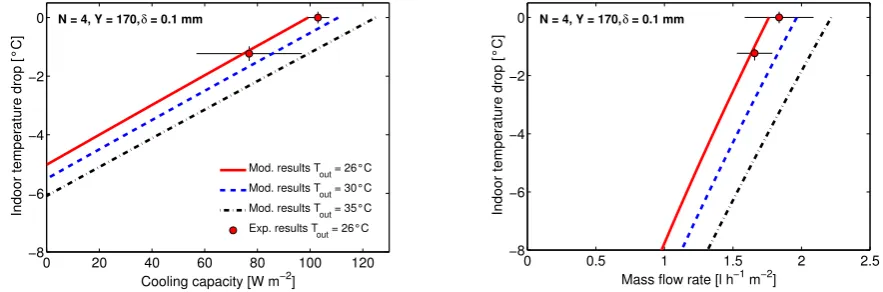
Effect of ambient temperature
Based on Antoine’s equation (see equation2.2), vapor pressure gradient and thus cooling capacity should increase with the operating temperature. In Figure10, we report the cooling performances as a function of both the temperature drop between indoor (i.e. thermal user) and ambient environments and the absolute ambient temperature (Tout). The latter is studied for values equal to 26◦C, 30◦C and
35◦C, respectively.
As expected, results show better cooling performances at higher ambient temperatures. It is interesting to highlight that, with typical summer conditions (Tout=35◦), the cooling power can reach
values up to 120Wm−2(at vanishing temperature difference).
0 20 40 60 80 100 120
−8 −6 −4 −2 0
Cooling capacity [W m−2]
Indoor temperature drop [°C]
Mod. results T
out = 26°C
Mod. results T
out = 30°C
Mod. results T
out = 35°C
Exp. results T
out = 26°C
N = 4, Y = 170, δ = 0.1 mm
0 0.5 1 1.5 2 2.5
−8 −6 −4 −2 0
Mass flow rate [l h−1 m−2]
Indoor temperature drop [°C]
N = 4, Y = 170, δ = 0.1 mm
Figure 10. Experimental and modeling performance of the cooling device with varying outdoor ambient temperature. (Left) Cooling capacity and (Right) specific mass flow rate are depicted. Modeling predictions are represented by colored lines, whereas experimental measures by red circles.
3.3. Ideal performances
The device prototype investigated in this work was only intended as a proof-of-concept and, as such, not optimally designed.
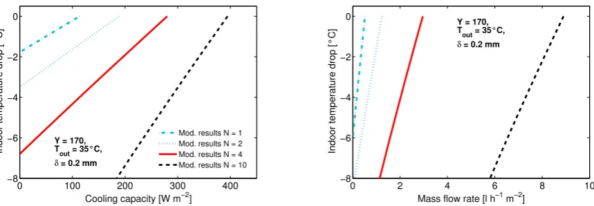
Nearly ideal device performance can be assessed by setting vanishing thermal resistances at both evaporator and condenser, an optimal thickness of the air gap between the two water solutions in each stage, and sufficiently high thermal transmittance at the top and bottom heat sinks.
Let us consider an ambient temperature of 35◦C, a salinity of 170 g/l and an air gap of≈0.2 mm in addition to the hydrophobic membrane. Let the number of stages be varied from 1 to 10. Results are presented in Figure11. As expected, the 10-stages setup achieves the highest cooling capacity, with maximum predicted values up to≈400Wm−2under the above favorable conditions. Clearly, this is
0 100 200 300 400 −8 −6 −4 −2 0
Cooling capacity [W m−2]
Indoor temperature drop [°C]
Mod. results N = 1 Mod. results N = 2 Mod. results N = 4 Mod. results N = 10 Y = 170,
T
out = 35°C,
δ = 0.2 mm
0 2 4 6 8 10
−8 −6 −4 −2 0
Mass flow rate [l h−1 m−2]
Indoor temperature drop [°C]
Y = 170, T
out = 35°C,
δ = 0.2 mm
Figure 11.Maximum modeling performances of the cooling device estimated with varying number of stages. (Left) Cooling capacity and (Right) specific mass flow rate are depicted. Modeling predictions are represented by colored lines.
4. Conclusions and discussion
A modular, static, low-cost and environmentally benign cooling device has been discussed and experimentally tested in this study. The device operation is possible without resorting to fluid circulation means or any moving mechanical parts: on the contrary, here we only rely on capillarity and gravity.
Experimental tests have been specifically carried out on a 4-stages lab-scale prototype, with ambient temperature kept close to 26◦C. The maximum cooling power measured in the experiments was≈103 ±4Wm-2(at vanishing temperature).
Experimental results are then used to validate a simplified one-dimensional theoretical model. This model was adopted to extrapolate the device behavior in wider range of possible configurations and operating conditions, aiming to define optimal values for future investigations.
As a future perspective, a fully passive solar cooling could be achieved by coupling the present device with a passive solar distiller, which is expected to provide both a steady distillate flow at the evaporator [4] and to restore the salinity at the condensed.
We stress that, in our specific realization, microporous hydrophobic membranes between the evaporator and condenser at each stage were needed to realize the hydraulic head between a unique saltwater basin and each condenser in the device, as schematically reported in Figure1. However, as done in [4], a membrane-free configuration can be also envisioned if, at each stage, the saltwater cavity is substituted by a hydrophilic layer holding the NaCl/water solution and a spacer is used to keep the two hydrophilic layers (evaporator and condenser) separated at a fixed distance. Clearly, in the latter case, the hydraulic head is no more possible, and each condenser should be served by a dedicated saltwater basin.
Author Contributions: E.C. conceived the idea of this study and supervised research activities. P.A. initially suggested the use of hydrophobic micro-porous membranes (MD) for sea water desalination, developed the theoretical model, suggested the use of finned heat sinks to improve the device performance and contributed to supervision of the work. M.M. engineered the prototype, conducted all experiments and simulations. M.F. helped with the prototype assembly, testing and supervision. All co-authors contributed to writing the paper.
Conflicts of Interest:The authors declare no conflict of interest.
References
2. F. Laganà, G. Barbieri, and E. Drioli, “Direct contact membrane distillation: modelling and concentration experiments,”Journal of Membrane Science, vol. 166, no. 1, pp. 1–11, 2000.
3. A. Alkhudhiri, N. Darwish, and N. Hilal, “Membrane distillation: a comprehensive review,”Desalination, vol. 287, pp. 2–18, 2012.
4. E. Chiavazzo, M. Morciano, F. Viglino, M. Fasano, and P. Asinari, “Performance analysis of a modular water distiller,”ArXiv:1702.05422, 2017.
5. E. Abu-Nada and H. F. Oztop, “Effects of inclination angle on natural convection in enclosures filled with cu–water nanofluid,”International Journal of Heat and Fluid Flow, vol. 30, no. 4, pp. 669–678, 2009.
c