Visualization of Thomas-Wigner Rotations

Visualization of Thomas-Wigner Rotations

Georg Beyerle ID

GFZ German Research Centre for Geosciences, Potsdam, Germany; [email protected]

Abstract: It is well known that a sequence of two non-collinear Lorentz boosts (pure Lorentz

1

transformations) does not correspond to a Lorentz boost, but involves a spatial rotation, the Wigner

2

or Thomas-Wigner rotation. We visualize the interrelation between this rotation and the relativity of

3

distant simultaneity by moving a Born-rigid object on a closed trajectory in several steps of uniform

4

proper acceleration. Born-rigidity implies that the stern of the boosted object accelerates faster than

5

its bow. It is shown that at least five boost steps are required to return the object’s center to its starting

6

position, if in each step the center is assumed to accelerate uniformly and for the same proper time

7

duration. With these assumptions, the Thomas-Wigner rotation angle depends on a single parameter

8

only. Furthermore, it is illustrated that accelerated motion implies the formation of an event horizon.

9

The event horizons associated with the five boosts constitute a natural boundary to the rotated

10

Born-rigid object and ensure its finite size.

11

Keywords:special relativity; Thomas-Wigner rotation; visualization

12

1. Introduction 13

In 1926 the British physicist L. H. Thomas (1903–1992) resolved a discrepancy between observed

14

line splittings of atomic spectra in an external magnetic field (Zeeman effect) and theoretical calculations

15

at that time [see e.g. 41]. Thomas’ analysis [39,40] explains the observed deviations in terms of

16

a special relativistic [9] effect. He recognized that a sequence of two non-collinear pure Lorentz

17

transformations (boosts) cannot be expressed as one single boost. Rather, two non-collinear boosts

18

correspond to a pure Lorentz transformation combined with a spatial rotation. This spatial rotation

19

is known as Wigner rotation or Thomas-Wigner rotation, the corresponding rotation angle is the

20

Thomas-Wigner angle [see e.g.2,4,5,14,15,17,18,24,27,28,30,32,34,36,42–44, and references therein].

21

The prevalent approach to discuss Thomas-Wigner rotations employs passive Lorentz

22

transformations. An objectGis simultaneously observed fromNinertial reference frames, denoted by

23

[1],[2], . . . ,[N]. Frame[i]is related to the next frame[i+1]by a pure Lorentz transformation, where

24

1≤i≤N−1. Now, for given non-collinear boosts from frame[1]to frame[2]and then from[2]to[3],

25

there exists a unique third boost from[3]to[4], such thatGis at rest with respect to both, frame[1]and

26

frame[4]. It turns out, however, that the combined transformation[1]→[2]→[3]→[4], is not the

27

identity transformation, but involves a spatial rotation.

28

In the present paper, following Jonsson [22], an alternative route to visualize Thomas-Wigner

29

rotations using active or “physical” boosts is attempted.Gis accelerated starting from zero velocity in

30

frame[1], which is denoted by “laboratory frame” in the following. During its journeyGperforms

31

several acceleration and/or deceleration manoeuvres and finally returns to its starting position. The

32

visual impression ofGmoving through the series of acceleration phases and finally coming to rest in a

33

rotated orientation (see fig.5below) hopefully outweigh the mathematical technicalities of the present

34

approach.

35

The paper is sectioned as follows. First, the general approach is described and basic assumptions

36

are introduced. The second section recalls uniform accelerations of Born-rigid objects. Sequences of

37

uniform, non-collinear accelerations for a given vertex point within a planar grid of vertices and the

38

trajectories of its neighbouring vertices are addressed in the following section. The last two sections

39

present the visualization results and discuss their implications. AppendixAexamines the required

40

number of boost steps, details of the computer algebraic calculations performed in this study are given

41

in appendixB.

42

For simplicity length units of light-seconds, abbreviated “ls” (roughly 300,000 km) are used with

43

the speed of light taken to be unity.

44

2. Method 45

We consider the trajectory of a square-shaped gridGconsisting ofMvertices.Gis assumed to be

46

Born-rigid, i.e. the distance between any two grid points, as observed in the momentarily comoving

47

inertial frame (MCIF) [see e.g.25, chapter 7], remains constant [3]. The grid’s central pointR, which

48

serves as the reference point, is uniformly accelerated for a given proper time period∆τR. To obtain 49

a closed trajectory several of these sections with constant proper acceleration, but different boost

50

directions are joined together.

51

InR’s MCIF the directions and magnitudes of the vertices’ proper accelerations~αi(i=1, . . . ,M) 52

change discontinuously at the switchover from one boost section to the next. In the MCIF the vectors~αi 53

change simultaneously; in other frames, such as the laboratory frame, the change is asynchronous and

54

G, despite its Born-rigidity, appears distorted and twisted (see fig.5below). On the other hand,G’s

55

Born-rigidity implies that it is sufficient to calculateR’s trajectory, the motion of the reference pointR 56

uniquely determines the trajectories of the remainingM−1 vertices [20,29]. We note that the spacetime

57

separations between individual switchover events, linking boost stepskandk+1, are spacelike. I.e.

58

these switchover events are causally disconnected and each vertex has to be “programmed” in advance

59

to perform the required acceleration changes [26].

60

In the following,αRand∆τRdenote the magnitude of the proper acceleration ofG’s reference 61

pointRand the boost duration in terms ofR’s proper time, respectively. To simplify the calculations

62

we impose the following four conditions on allNboosts.

63

1. The gridGis Born-rigid.

64

2. At the beginning and after completion of theNth boostGis at rest in frame[1]andRreturns to

65

its starting position.

66

3. R’s proper accelerationαRand the boost’s proper duration∆τRare the same in allNsections. 67

4. All boost directions and therefore all trajectories lie within thexy-plane.

68

Let the unit vector ˆe1denote the direction of the first boost in frame[1]. This first boost lasts for a

69

proper time∆τR, as measured byR’s clock, whenRattains the final speedvR ≡ βwith respect to 70

frame[1]. Frame[2]is then defined asR’s MCIF at this instant of time. The corresponding Lorentz

71

matrix transforming a four-vector from frame[2]to frame[1]is

72

Λ(γ, ˆe1)≡



 

γ, γ βeˆT₁ γ βeˆ1, 13×3+ (γ−1)eˆ1·eˆT1





 . (1)

Here,13×3is the 3×3 unit matrix, the superscriptTdenotes transposition, the Lorentz factor is

73

γ≡ p 1

1−β2

(2)

and, in turn,β=pγ2−1/γ. Similarly, frame[3]isR’s MCIF at the end of the second boost, etc. In 74

general, the Lorentz transformation from frame[i]to frame[i+1]is given by eqn. (1), with ˆe1replaced

75

by ˆei, the direction of theith boost in frame[i]. 76

Assumption {3} implies that the angles between consecutive boosts (“boost angles”)

77

ζi,i+1 ≡ arccos

ˆ

eT_i ·eˆi+1

are the only unknowns, since proper accelerationαRand boost duration∆τRare given parameters. In 78

the following the “half-angle” parametrization

79

T≡tan

ζ 2

(4)

is used; it allows us to write expressions involving

80

sin(ζ) = 2T

1+T2 (5)

cos(ζ) = 1−T 2

1+T2 . as polynomials inT.

81

We will find that, first, no solutions exist if the number of boostsNis four or less (see appendixA),

82

second, forN=5 the solution is unique and, third, the boost anglesζ(γ)depend solely on the selected

83

value ofγ=1/p1−β2. ChangingαRand/or∆τRonly affects the spatial and temporal scale ofR’s 84

trajectory (see below).

85

The derivation ofζi,i+1(γ)is simplified by noting that the constraints {2}, {3} and {4} imply time

86

reversal invariance. I.e.R’s trajectory from destination to start, followed backward in time, is a valid

87

solution as well and thereforeζi,i+1=ζN−i,N−i+1fori=1, . . . ,N−1. Thus, forN=5 the number of

88

unknowns reduces from four to two, withζ1,2=ζ4,5andζ2,3=ζ3,4. 89

3. Uniform acceleration of a Born-rigid object 90

In the laboratory frame we consider the uniform acceleration of the reference pointR, initially

91

at rest, and assume that the acceleration phase lasts for the proper time period∆τR. During∆τRthe 92

reference point moves from location~rR(0)to location

93

~rR(∆τR) = ~rR(0) + 1 αR

(cosh(αR∆τR)−1)eBˆ (6)

with unit vector ˆeB denoting the boost direction [see e.g.19,21,27,33,36,37]. The coordinate time

94

duration∆tRcorresponding to the proper time duration∆τRis 95

∆tR =

1 αR

sinh(α_R∆τR) (7)

andRattains the final speed

96

vR=tanh(αR∆τR) =β . (8)

LetGbe an arbitrary vertex point ofGat location~rG(0)and

97

b≡(~rG(0)−~rR(0))·eBˆ (9)

the projection of the distance vector fromRtoGonto the boost direction ˆeB. The verticesGandRstart

98

to accelerate simultaneously sinceGis Born-rigid (assumption {1}) and analogous to eqns. (6), (7) and

99

(8) we obtain forG’s trajectory

100

~rG(∆τG) = ~rG(0) +

1 αG

(cosh(αG∆τG)−1) +b

ˆ

eB (10)

∆tG = 1

αG sinh

(αG∆τG)

At the end of the first boost phase all grid points move at the same speed with respect to the laboratory

101

frame; however, in the laboratory frame the boost phase does not end simultaneously for all vertices.

102

Simultaneity is only observed inR’s MCIF. WithvG=vRand eqn. (10) it follows

103

αG∆τG = αR∆τR . (11)

G’s Born-rigidity implies that the spatial distance betweenGandRat the end of the boost phase inR’s

104

MCIF is the same as their distance at the beginning of the boost phase. A brief calculation leads to

105

− 1 αG

(γ−1) +bγ+ 1 αR

(γ−1) =b (12)

which simplifies to

106

αG = 1

1+bαR

αR (13)

and with eqn. (11)

107

∆τG = (1+bαR)∆τR (14)

provided γ 6= 1. Eqn. (13) expresses the well-known fact that the proper accelerations aboard a 108

Born-rigid grid may differ from one vertex to the next. More specifically, at a location trailing the

109

reference pointRthe acceleration exceedsαR, vertex points leadingRaccelerate less thanαR. (In 110

relativistic space travel the passengers in the bow of the spaceship suffer lower acceleration forces than

111

those seated in the stern. This amenity of a more comfortable acceleration, however, is counterbalanced

112

by faster ageing of the space travellers (eqn. (14)). These considerations, of course, assume Born-rigidly

113

constructed space vehicles.)

114

The position-dependent acceleration is well-known from the Dewan-Beran-Bell spaceship paradox

115

[7,8] and [1, chapter 9]. Two spaceships, connected by a Born-rigid wire, accelerate along the direction

116

separating the two. According to eqn. (13) the trailing ship has to accelerate faster than the leading

117

one. Conversely, if both accelerated at the same rate in the laboratory frame, Born-rigidity could

118

not be maintained and the wire connecting the two ships would eventually break. This well-known,

119

but admittedly counterintuitive fact is not a paradox in the true sense of the word and discussed

120

extensively in the literature [see e.g.11–13,16,31,38].

121

Eqns. (13) and (14) also imply, thatαG →∞and∆τG →0, as the distance between a (trailing) 122

vertexGand the reference pointRapproaches the critical value

123

b∗≡ −1/αR . (15)

Clearly, a Born-rigid object cannot extend beyond this boundary, which is referred to as “event horizon”

124

in the following. Section6.2will discuss its consequences.

125

Finally, we note that eqn. (14) implies that a set of initially synchronized clocks mounted on

126

a Born-rigid grid will in general fall out of synchronization once the grid is accelerated [37]. Thus,

127

the switchover events, which occur simultaneous inR’s MCIF, are not simultaneous with respect to

128

the time displayed by the vertex clocks. As already mentioned, the acceleration changes have to be

129

“programmed” into each vertex in advance, since the switchover events are causally not connected and

130

lie outside of each others’ lightcones [10].

131

4. Sequence of five uniform accelerations 132

The previous section discussedR’s trajectory during the first acceleration phase (eqn. (10)). Now

133

we connect several of these segments to form a closed trajectory forR. Let A[k]denoteR’s start event

134

as observed in frame[k]and B[k], C[k], etc. correspondingly denote the “switchover” events between 1st

and 2stboost, 2ndand 3rdboost, etc., respectively. In the following, bracketed superscripts indicate the

136

reference frame. Frame[1], i.e.k=1, is the laboratory frame, frame[2]is obtained from frame[1]by

137

the Lorentz transformationΛ(γ,−eˆ1)(eqn. (1)). Generally, frame[k+1]is calculated from frame[k]

138

using the transformation matrixΛ(γ,−ekˆ ).

139

It can be shown (see appendix A) that at least five boosts are needed to satisfy the four

140

assumptions {1}–{4} listed in section2. As illustrated in fig.3for a sequence ofN = 5 boosts the

141

reference point starts to accelerate at event A and returns at event F via events B, C, D and E. The

142

corresponding four-positionPand four-velocityVare

143

P[_F1] = P_A[1]+S[_A1]_→B (16)

+Λ(γ,−eˆ1)·S[B2→] C

+Λ(γ,−eˆ1)· Λ(γ,−eˆ2)·S[_C3→] D

+Λ(γ,−eˆ1)· Λ(γ,−eˆ2)· Λ(γ,−eˆ3)· S[_D4]→E

+Λ(γ,−eˆ1)· Λ(γ,−eˆ2)· Λ(γ,−eˆ3)· Λ(γ,−eˆ4)· S[E5→] F and

144

V[_F1] = Λ(γ,−eˆ1)· Λ(γ,−eˆ2)· Λ(γ,−eˆ3) (17) ·Λ(γ,−eˆ4)· Λ(γ,−eˆ5)· V[_F6] ,

respectively. Here, the four-vector

145

S[_A1]_→B ≡ 1 αR

sinh(αR∆τR) (cosh(αR∆τR)−1)eˆ1

!

(18)

= 1

αR

γ β (γ−1)eˆ1

!

describes R’s worldline from A to B (eqn. (10)); S[_B2_→] _C, S_C[3_→] _D, S[_D4_→] _E and S[_E5_→] _F are defined

146

correspondingly. Assumption {2} implies that

147

~

P_A[1]=~P_F[1]=~P_A[6]=~P_F[6] =~0 (19) and

148

V_A[1]=V[_F1] =V_A[6]=V[_F6]= _~1 0

!

. (20)

To simplify the expressions in eqns. (16) and (17) time reversal symmetry is invoked. It implies that

149

the set of boost vectors−eˆ5,−eˆ4, . . . ,−eˆ1constitutes a valid solution, provided ˆe1, ˆe2, . . . , ˆe5is one and

150

satisfies assumptions {1}–{4}. Thereby the number of unknowns is reduced from four to two, the angle

151

between the boost vectors ˆe1and ˆe2, and the angle between ˆe2and ˆe3

152

ζ1,2 ≡ arccos

ˆ

eT₁ ·eˆ2

=arccoseˆ₄T·eˆ5

(21)

ζ2,3 ≡ arccos

ˆ

eT₂ ·eˆ3

=arccoseˆ₃T·eˆ4

.

Fig.3illustrates the sequence of the five boosts in the laboratory frame[1]. Since the start and final

153

velocities are zero, R’s motion between A and B and, likewise, between E and F is rectilinear. In

154

contrast, the trajectory connecting B and E (via C and D) appears curved in frame[1]; as discussed

and illustrated below, the curved paths are in fact straight lines in the corresponding boost frame (see

156

fig.4).

157

From eqns. (17) and (20) follows

(T12)2−2γ−1

(T23)2−4(1+γ)T12T23+ (T12)2+4γ2+2γ−1=0 (22) with the two unknownsT12≡tan(ζ1,2/2)andT23≡tan(ζ2,3/2)(for details see appendixB). Eqn. (22)

158

has two solutions,

159

T₂₃(±) = 1

−(T12)2+2γ+1 (23)

×

−2T12 (γ+1)

±q−(T12)4+8(T12)2γ+6(T12)2+8γ3+8γ2−1

provided

160

(T12)2−2γ−16=0 . (24)

Assumption {2} implies that the spatial component of the eventP[_F1]vanishes, i.e.

161

~

P_F[1]=0 . (25)

Since all motions are restricted to thexy-plane, it suffices to consider thex- andy-components of

162

eqn. (25). They-component leads to a product of the following two expressions

163

(T12)8 (26)

+(T12)64 (γ+2) +(T12)4(−2) (2γ+1)

2γ2+8γ+9

+(T12)2(−4)

8γ4+28γ3+26γ2+5γ−2

−(2γ+1)3

4γ2+2γ−1

or

164

(T12)8 (γ+3)2 (27)

+(T12)6(−4)

6γ3−15γ2−12γ+5

+(T12)4(−2)

24γ4−44γ3−55γ2+26γ+1

+(T12)2(−4)

8γ5−16γ4−14γ3+5γ2+1

+4γ2+γ−1

2

(see appendixB). The solutions of equating expression (27) to zero are disregarded since forγ=1 it 165

yields

166

(T12)8+4(T12)6+6(T12)4+4(T12)2+1=0 (28) which has no real-valued solution forT12.

It turns out (see appendixB) that thex-component of eqn. (25) results in an expression containing

168

two factors as well, one of which is identical to the expression (26). Thus, the roots of the polynomial (26)

169

solve eqn. (25).

170

The degree of the polynomial (26) in terms of(T12)2is four; its roots are classified according

171

to the value of the discriminant∆ (see e.g. en.wikipedia.org/wiki/Quartic_function), which for

172

expression (26) evaluates to

173

∆ = −524288γ(γ−1)3(γ+1)7(4γ4+28γ3+193γ2+234γ+81) . (29)

For non-trivial boostγ>1, the discriminant is negative and the roots of the quartic polynomial consist 174

of two pairs of real and complex conjugate numbers (seeen.wikipedia.org/wiki/Quartic_function).

175

The real-valued solutions are

176

(T12)2 = −(γ+2) +S+ 1 2

r

−4S2_−2p− q

S (30)

and

177

T₁₂(b)2 = −(γ+2) +S −1 2

r

−4S2_−2p− q

S (31)

with

178

p ≡ −2(γ+1) 4γ2+17γ+21

(32)

q ≡ −16(γ+1)γ2−2γ−9

S ≡ 1

2√3

r

−2p+Q+∆0 Q

∆0 ≡ 16(γ+1)2 4γ4+28γ3+157γ2+126γ+9

Q ≡ 4 3

q

Q0+12 √

6pQ0

Q0 ≡ γ(γ−1)3(γ+1)7(4γ4+28γ3+193γ2+234γ+81) .

The solution from eqn. (31) turns out to be negative and thus does not produce a real-valued solution

179

forT12. The remaining two roots of the polynomial (26)

180

T₁₂(c)2 = −(γ+2)− S+1 2

r

−4S2_−2p+ q

S (33)

T₁₂(d)2 = −(γ+2)− S −1 2

r

−4S2_−2p+ q S

correspond to replacingS by−S in eqns. (30) and (31); they are complex-valued and therefore

181

disregarded as well. The second unknown,T23, follows from eqn. (23) by choosing the positive square

182

root+p(T12)2and using

183

T23 ≡ T23(+) (34)

(see eqn. (22)). For a given Lorentz factorγthe angles between the boost directions ˆeiand ˆei+1are

184

ζ1,2(γ) = arccos

ˆ

eT₁ ·eˆ2

=2 arctan

+

q

(T12(γ))2

(35)

ζ2,3(γ) = arccos

ˆ

eT₂ ·eˆ3

=2 arctan

+

q

(T23(γ))2

10

10

10

10

10

10

γ

50

75

100

125

150

175

200

ζ

,

ζ

[deg]

Figure 1. The angle between the boost direction vectors ˆe1and ˆe2in frame[1](blue line), and the angle

between ˆe2and ˆe3in frame[2](red) as a function ofγ. The dotted line marks+180◦, the limit ofζ1,2

andζ2,3forγ→∞.

and, withζ4,5=ζ1,2andζ3,4 =ζ2,3, the orientation of the five boost directions ˆeifori=1, . . . , 5 within 185

thexy-plane are obtained.

186

Fig.1shows numerical values of the boost anglesζ1,2(γ)andζ2,3(γ)as a function ofγ. The angles increase from

ζ1,2(γ=1) =2 arctan

q

−5+4√10

≈140.2◦

and

ζ2,3(γ=1) =2 arctan

p

−5+4√10−√3p−5+2√10 −2+√10

!

≈67.2◦

atγ=1 toζ1,2(γ→∞) = +180◦=ζ2,3(γ→∞)asγ→∞. 187

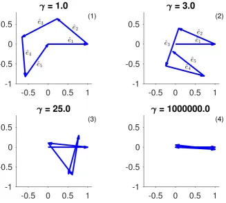
Fig.2depicts the orientation of the five boost directions for several values ofγ. Here the first boost 188

vector ˆe1is taken to point along thex-axis. We note that the panels in fig.2do not represent a specific

189

reference frame; rather, each vector ˆekis plotted with respect to frame[k](k = 1, . . . , 5). The four 190

panels show the changes in boost directions for increasing values ofγ. Interestingly, the asymptotic 191

limitsζ1,2(γ→∞) = +180◦andζ2,3(γ→∞) = +180◦imply that in the relativistic limitγ→∞the 192

trajectory ofRessentially reduces to one-dimensional motions along thex-axis. At the same time the

193

Thomas-Wigner rotation angle increases to+360◦asγ→∞(see the discussion in section6below). 194

Since the accelerated object is Born-rigid, the trajectories of all grid verticesG are uniquely

195

determined once the trajectory of the reference pointRis known [10,20,29]. Following the discussion in

196

section3the position and coordinate time of an arbitrary vertexG, in the frame comoving withRat the

-0.5

0

0.5

1

-1

-0.5

0

0.5

= 1.0

(1)

-0.5

0

0.5

1

-1

-0.5

0

0.5

= 3.0

(2)

-0.5

0

0.5

1

-1

-0.5

0

0.5

= 25.0

(3)

-0.5

0

0.5

1

-1

-0.5

0

0.5

= 1000000.0

Figure 2. Boost directions for four different values ofγ=1/p1−β2. The boost direction in frame[1],

ˆ

e1is assumed to point along thex-axis. In the relativistic limitγ→∞(panel (4)) the angles between

ˆ

ek and ˆek+1 approach+180◦ and the motion of the reference pointRtends to be more and more

0

0.1

0.2

0.3

0.4

x [ls]

-0.05

0

0.05

0.1

0.15

0.2

0.25

0.3

y [ls]

B[1]

C[1] D[1]

E[1]

B[6]

C[6]

D[6]

E[6]

A[1]=F[1], A[6]=F[6]

[1] [6]

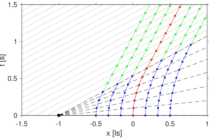
Figure 3. Trajectories of reference pointRforγ=2/ √

3≈1.15 as seen from (laboratory) frame[1]and frame[6]. The two frames are stationary with respect to each other, but rotated by a Thomas-Wigner angle ofθTW=14.4◦.

beginning of the corresponding acceleration phase, follows from eqn. (10). The resulting trajectories

198

are discussed in the next section.

199

5. Visualization 200

The trajectory of the reference point R in the laboratory frame for a boost speed β = 1/2, 201

corresponding toγ=2/ √

3≈1.15, is displayed in fig.3(black solid line). The same trajectory as it

202

appears to an observer in frame[6]is marked in grey. The two frames are stationary with respect to

203

other, but rotated by a Thomas-Wigner angle of about 14.4◦. In addition, dots mark the locations of the

204

four switchover events B, C, D and E in the two frames. As required by assumption {2} the starting

205

and final positions, corresponding to the events A and F, coincide.

206

Fig.4shows the same trajectory as fig.3. In addition,R’s trajectories as recorded by observers

207

in the frames[2], . . . ,[5]are plotted as well (solid coloured lines). Corresponding switchover events

208

are connected by dashed lines. At B[2], C[3], D[4] and E[5] (and of course at the start event A[1,6]

209

and destination event F[1,6]) the reference pointRslows down and/or accelerates from zero velocity

210

producing a kink in the trajectory. In all other cases the tangent vectors of the trajectories, i.e. the

211

velocities are continuous at the switchover points.

212

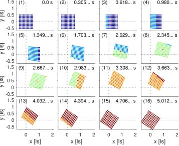
With eqns. (30) and (34) all necessary ingredients to visualize the relativistic motion of a Born-rigid

213

object are available. In fig.5the object is modelled as a square-shaped grid of 11×11 points, arranged

214

around the reference pointR. The object uniformly accelerates in thexy-plane changing the boost

215

direction four times by the anglesζ1,2 (as measured in frame [2]),ζ2,3 (frame[3]),ζ2,3 (frame[4])

216

and finallyζ1,2(frame[5]). The vertices’ colour code indicates the corresponding boost section. The

-2

-1.5

-1

-0.5

0

0.5

1

1.5

x [ls]

-1

-0.5

0

0.5

1

1.5

y [ls]

B[2] C[2] D[2]

E[2] F[2]

B[3] C[3] D[3]

E[3]

F[3]

B[4] C [4] D

[4]

E[4] F[4] B[5]

C[5] D[5] E[5]

F[5]

frame [1]

frame [2]

frame [3]

frame [4]

frame [5]

frame [6]

Figure 4. Trajectories of the reference pointRas seen from the six reference frames[1],[2], . . . ,[6]. The switchover points are marked byX[_ik]withX=A, . . . , F. Corresponding switchover points are connected by dashed lines. The Lorentz factor isγ=2/

√

-0.5 0 0.5 1 1.5

y [ls]

0.0 s (1)

-0.5 0 0.5 1 1.5

y [ls]

1.349... s (5)

-0.5 0 0.5 1 1.5

y [ls]

2.667... s (9)

0 1 2

x [ls]

0 0.5 1 1.5

y [ls]

4.032... s (13)

0.305... s (2)

1.703... s (6)

2.983... s (10)

0 1 2

x [ls]

0.618... s (3)

2.029... s (7)

3.308... s (11)

0 1 2

x [ls]

0.980... s (4)

2.345... s (8)

3.663... s (12)

0 1 2

x [ls]

Figure 5. A series of grid positions as seen in the laboratory frame. The boost speed is taken to be

β =0.7, resulting in a Thomas-Wigner rotation angle of about 33.7◦. Coordinate time is displayed

16 panels depict the grid positions in the laboratory frame[1]for specific values of coordinate time

218

displayed in the top right.

219

To improve the visual impression the magnitude of the Thomas-Wigner rotation in fig.5is

220

enlarged by increasing the boost speed fromβ=0.5, used in figs.3and4, toβ=0.7 corresponding 221

toγ≈1.4. Despite appearance the gridG is Born-rigid, inR’s MCIF the grid maintains its original 222

square shape. In the laboratory frame, however,Gappears compressed, when it starts to accelerate

223

or decelerate and sheared, when one part ofG has not yet finished boostk, but the remaining part

224

ofG already has transitioned to the next boost sectionk+1. This feature is clearly evident from

225

panels (4), (7), (10) or (13) in fig.5with the occurrence of two colours indicating two boost sections

226

taking effect at the same epoch of coordinate laboratory time. We note, however, that the switchover

227

events occur simultaneously for all grid points inR’s MCIF. The non-uniform colouring illustrate the

228

non-simultaneity of the switchovers in the laboratory frame and thereby the relationship between

229

Thomas-Wigner rotations and the non-existence of absolute simultaneity.

230

6. Discussion 231

In this final section the Thomas-Wigner rotation angle is calculated from the known boost

232

angles ζ1,2(γ) and ζ2,3(γ) (eqn. (35)). In addition, the maximum diameter of Born-rigid objects,

233

Thomas-Wigner-rotated by a series of boosts, is discussed.

234

6.1. Derivation of Thomas-Wigner angle 235

From the preceding sections follows a straightforward calculation of the Thomas-Wigner angle

236

as a function of Lorentz factor γ. Assumption {2} implies that the sequence of the five Lorentz 237

transformations[6]→[5]→. . .→[1]is constructed such that frame[6]is stationary with respect to

238

frame[1]and their spatial origins coincide. I.e. the combined transformation reduces to an exclusively

239

spatial rotation and the corresponding Lorentz matrix can be written as

240

Λ(γ,−eˆ1)· Λ(γ,−eˆ2)· Λ(γ,−eˆ3)· Λ(γ,−eˆ4)· Λ(γ,−eˆ5) =



   

1 0 0 0

0 R1,1 R1,2 R1,3 0 R2,1 R2,2 R2,3 0 R3,1 R3,2 R3,3



   

. (36)

Since the rotation is confined to thexy-plane, the matrix elementsR3,i =0=Ri,3withi=1, 2, 3 vanish.

241

The remaining elements

242

R1,1(γ) = R2,2(γ)≡cos(θTW(γ)) (37)

R1,2(γ) = −R2,1(γ)≡sin(θTW(γ))

yield the Thomas-Wigner rotation angleθTW 243

˜

θTW(γ) ≡ atan2(R2,1(γ),R1,1(γ)) (38)

θTW(γ) ≡

(

˜

θTW(γ) : θ˜TW(γ)≥0

˜

θTW(γ) +2π : θ˜TW(γ)<0

with atan2(·,·)denoting the four-quadrant inverse tangent. Eqn. (38) ensures that angles exceeding

244

+180◦are unwrapped and mapped into the interval[0◦,+360◦](see fig.6).

With eqn. (36) the rotation matrix elementsR1,1andR2,1are found to be (see appendixB)

246

R1,1(γ) = −1+

(γ+1)

((T12)2+1)4((T23)2+1)4

(39)

×

(T12)4(T23)4+2(T12)4(T23)2+ (T12)4

−4(T12)3(T23)3γ+4(T12)3(T23)3−4(T12)3T23γ +4(T12)3T23−2(T12)2(T23)4γ+4(T12)2(T23)4 +4(T12)2(T23)2γ2+8(T12)2(T23)2γ−8(T12)2(T23)2 −4(T12)2γ2+10(T12)2γ−4(T12)2

+12T12(T23)3γ−12T12(T23)3−16T12T23γ2 +12T12T23γ+4T12T23+2(T23)4γ

−(T23)4−4(T23)2γ2+6(T23)2+4γ2−2γ−1

2

and

247

R2,1(γ) = 4

(γ−1) (γ+1)

((T12)2+1)4((T23)2+1)4

(40)

×

(T12)3(T23)2+ (T12)3+3(T12)2(T23)3 −2(T12)2T23γ+ (T12)2T23+T12(T23)4 −2T12(T23)2γ−3T12(T23)2+2T12γ −(T23)3+2T23γ+T23

×

(T12)4(T23)4+2(T12)4(T23)2+ (T12)4

−4(T12)3(T23)3γ+4(T12)3(T23)3−4(T12)3T23γ +4(T12)3T23−2(T12)2(T23)4γ+4(T12)2(T23)4 +4(T12)2(T23)2γ2+8(T12)2(T23)2γ−8(T12)2(T23)2 −4(T12)2γ2+10(T12)2γ−4(T12)2

+12T12(T23)3γ−12T12(T23)3−16T12T23γ2 +12T12T23γ+4T12T23+2(T23)4γ

−(T23)4−4(T23)2γ2+6(T23)2+4γ2−2γ−1

withT12=T12(γ)andT23 =T23(γ)given by eqns. (30) and (34), respectively.

248

The resulting angleθTW(γ)as a function ofγis plotted in fig.6. The plot suggests thatθTW → 249

+360◦asγ → ∞. As already mentioned in subsection4(see fig.2) the boost anglesζ1,2 →+180◦

250

andζ2,3 → +180◦in the relativistic limitγ → ∞. Notwithstanding thatR’s trajectory reduces to 251

an one-dimensional motion asγ →∞, the grid’s Thomas-Wigner rotation angle approaches a full 252

revolution of+360◦in the laboratory frame.

253

6.2. Event horizons 254

As illustrated by fig.5the Born-rigid objectGrotates in thexy-plane. Clearly, in order to preclude

255

paradoxical faster-than-light translations of sufficiently distant vertices,G’s spatial extent in thex- and

256

y-directions has to be bounded by a maximum distance from the reference pointRon the order of

10

10

10

10

10

10

γ

0

60

120

180

240

300

360

θ

[deg]

Figure 6. Thomas-Wigner rotation angle as a function ofγ. For clarity the angle is unwrapped and

-1.5

-1

-0.5

0

0.5

1

x [ls]

0

0.5

1

1.5

t [s]

Figure 7. Spacetime diagram of a one-dimensional grid consisting of seven points. The grid accelerates towards the positivex-direction. The trajectories are marked in blue/green, the mid point is taken as the referenceRand its worldline is colored in red. Dots indicate the lapse of 0.1 s in proper time. After 0.6 s have passed onR’s clock, the acceleration stops and the points move with constant speed (green lines). Dashed and dotted lines connect simultaneous spacetime events inR’s comoving frame.

∆t/θTW[3]. As discussed in the following, this boundary is put into effect by event horizons associated 258

withG’s acceleration in each of the five boosts.

259

Fig. 7exemplifies the formation of an event horizon for an accelerated object in 1+1 (one

260

time and one space) dimensions [see e.g. 6,10,19,35]. Here, the Born-rigid object is assumed to

261

be one-dimensional and to consist of seven equidistant grid points. Each point accelerates for a

262

finite time period towards the positivex-direction (blue worldlines); the reference pointR, marked

263

in red, accelerates withαR ≡ 1 ls/s2. Contrary to the simulations discussed in fig.5above, for 264

illustrative purposes the acceleration phase is not followed immediately by another boost. Rather,

265

the object continues to move with constant speed after the accelerating force has been switched off

266

(green worldlines in fig.7). The completion of the acceleration phase is synchronous inR’s MCIF

267

(dashed-dotted line) and asynchronous in the laboratory frame. Fig. 7also illustrates that for an

268

uniform acceleration the event horizon (black dot) is stationary with respect to the laboratory frame.

269

In this simulation each vertex is assumed to be equipped with an ideal clock ticking at a proper

270

frequency of 10 Hz, the corresponding ticks are marked by dots; the boost phase lasts for 0.6 s onR’s

271

clock. The clocks of the left-most (trailing) and right-most (leading) vertex measure (proper time) boost

272

durations of 0.3 s and 0.9 s, respectively. Thus, with respect to the MCIFs (dashed lines) the vertex

273

clocks run at different rates (see eqn. (14)). The trailing clocks tick slower, the leading clocks faster

274

than the reference clock atR. From eqns. (13) and (14) it follows that the proper time variations are

275

compensated by corresponding changes in proper acceleration experienced by the seven vertices. For

the numerical values used in fig.7the accelerations of the trailing and leading vertex are 2αRand 277

2αR/3, respectively. 278

The spatial components of the inertial reference frames, comoving withR, are plotted in fig.7as

279

well. During the acceleration-free period following the boost phase the grid moves with constant speed

280

and the equal-time slices of the corresponding comoving frames (dotted lines) are oriented parallel to

281

other. During the boost phase, however, the lines intersect and eqn. (10) entails that the equal-time

282

slices of the comoving frames all meet in one spacetime point, the event horizonxH≡ −1 ls (black dot

283

atx=−1 ls andt=0 s in fig.7).

284

If the accelerating grid extended toxH, the corresponding vertex would experience infinite proper

285

acceleration (eqns. (13) and (14)) and its clock would not tick. Clearly, a physical object accelerating

286

towards positivex(fig.7) cannot extend beyond this boundary atxH. If the grid in fig.7is regarded

287

as realization of an accelerating coordinate system, this frame is bounded in the spatial dimension

288

and ends at the coordinate valuexH. However, as soon as the grid’s acceleration stops, the event

289

horizon disappears and coordinatesx<xHare permissible. We note, that the event horizon in fig.7 290

is a zero-dimensional object, a point in 1+1-dimensional spacetime considered here. The horizon is

291

frozen in time and exists only for the instantt=0.

292

Generalizing this result we find that the five boosts described in subsection4and depicted in

293

fig.3induce five event horizons in various orientations. It turns out that the accelerated objectGis

294

bounded by these horizons in all directions within thexy-plane. They limitG’s maximum size [3] and

295

thereby assure that all of its vertices obey the special relativistic speed limit [9].

296

7. Conclusions 297

It is well known that pure Lorentz transformations do not form a group in the mathematical sense,

298

since the composition of two transformations in general is not a pure Lorentz transformation again,

299

but involves the Thomas-Wigner spatial rotation. The rotation is visualized by uniformly accelerating

300

a Born-rigid object, consisting of a finite number of vertices, such that the object’s reference point

301

returns to its starting location. It turns out that at least five boosts are necessary, provided, first, the

302

(proper time) duration and the magnitude of the proper acceleration is the same within each boost

303

and, second, the object’s motion is restricted to thexy-plane. Analytic expressions are derived for the

304

angles between adjacent boost directions.

305

The visualization illustrates the relationship between Thomas-Wigner rotations and the relativity

306

of simultaneity. The transition from one boost section to the next occurs synchronously in the MCIF

307

of the object’s reference point. In the laboratory frame, however, the trailing vertices perform the

308

transition to the next boost phase, which in general involves a direction change, earlier than the

309

leading vertices. Thus, in this frame the accelerated object not only contracts and expands along

310

its direction of propagation, but also exhibits a shearing motion during the switchover phases. The

311

simulations illustrate clearly that the aggregation of these shearing contributions finally adds up to the

312

Thomas-Wigner rotation.

313

Accelerated motions induce event horizons, which no part of a physical, Born-rigid object may

314

overstep. Thus, the object’s size is limited to a finite volume or area (if its motion is restricted to two

315

spatial dimension) and Thomas-Wigner rotations by construction observe the special relativistic speed

316

limit.

317

Acknowledgments: Several calculations of this study were performed with the computer algebra system “SymPy”

318

[23], available at the URLwww.sympy.org. “SymPy” is licensed under the General Public License; for more

319

information seewww.gnu.org/licenses/gpl.html. All trademarks are the property of their respective owners.

320

Supplementary Materials: An MPEG-4 video animation of the Thomas-Wigner rotation, the MATLABsource

321

code used to create fig.5and the “SymPy” script file discussed in appendixBare available at the URLwww. 322

gbeyerle.de/twr.

323

Conflicts of Interest:The author declares no conflict of interest.

324

MCIF momentarily comoving inertial frame

326

Appendix A Number of boosts 327

We determine the smallest number of boosts that satisfies the four assumptions listed in section2.

328

Denoting the number of boosts byN, it is self-evident thatN≥3, since forN=1 the requirement of

329

vanishing final velocity cannot be met ifvR6=0. And forN=2 the requirement of vanishing final

330

velocity implies collinear boost directions. With two collinear boosts, however, the reference pointR 331

does not move along a closed trajectory. In addition, we note, that collinear boosts imply vanishing

332

Thomas-Wigner rotation [see e.g.36].

333

Appendix A.1 Three boosts 334

Consider three boosts of the reference pointRstarting from location A and returning to location D

335

via locations B and C. In the laboratory frame (frame[1]) the four-position at the destination D is given

336

by

337

P[_D1] = P_A[1]+S_A[1_→] _B (A1)

+Λ(γ,−eˆ1)· S[B2→] C

+Λ(γ,−eˆ1)· Λ(γ,−eˆ2)· S[C3→] D and

338

V_D[1] = Λ(γ,−eˆ1)· Λ(γ,−eˆ2)· Λ(γ,−eˆ3)· V[_D4] (A2) is the corresponding four-velocity. For the definition of the four-vector S[_A1]_→B see eqn. (18).

339

Assumption {2} implies that

340

~

P_A[1]=~P_D[1]=~P_A[4]=~P_D[4] =~0 (A3) and

341

V_A[1]=V[_D1] =V_A[4]=V[_D4]= _~1 0

!

. (A4)

Inserting eqn. (1) into eqn. (A2) yields

342

T12 = T23 =±

p

2γ+1 (A5)

(see appendixB) and, in turn, using eqn. (A3) we obtain

343

~

P_D[1]= 1 (γ+1)2



 

−(γ−1)2(2γ+1)2 −(γ−1) (2γ+1)

3

2 (3_γ+1)

0



 

!

=~0 . (A6)

Its only solution for real-valuedβis the trivial solutionγ=1, i.e.β=0. Thus, there are no non-trivial 344

solutions forN=3 boosts, which are consistent with the assumptions {1}-{4}.

345

Appendix A.2 Four boosts 346

For a sequence of four boosts time reversal symmetry implies thatR’s velocity in the laboratory

347

frame vanishes at event C after the second boost, i.e.~VC[1]=~0. However, stationarity in the laboratory

frame can only be achieved if the first two boosts A→B and B→C are collinear. In order to fulfil

349

assumption {2} the third and fourth boosts have to be collinear with the first (and second) boost

350

as well. As already noted, a sequence of collinear boosts, however, does not produce a non-zero

351

Thomas-Wigner rotation.

352

Appendix B Computer algebra calculations 353

Some equations in this paper were derived using the computer algebra system “SymPy” [23].

354

The corresponding “SymPy” source code filesvtwr3bst.py(three boost case, see sectionA.1) and

355

vtwr5bst.py(five boost case, see section4) are available for download atwww.gbeyerle.de/twr. These

356

scripts process eqns. (A1), (A2), (16) and (17) and derive the results given in eqns. (A5), (A6), (23), (26),

357

(27), (39) and (40). The following paragraphs provide a few explanatory comments.

358

First, we address the case of three boosts (superscript(3B)) and the derivation of eqn. (A5). The

359

corresponding boost vectors in thexy-plane ˆe(_i3B)withi=1, 2, 3 are taken to be

360

ˆ

e(₁3B)≡ Ca Sa

!

= 1

1+ (T12)2

1−(T12)2 2T12

!

(A7)

ˆ

e(₂3B)≡ 1 0

!

ˆ

e(₃3B)≡ Ca −Sa

!

= 1

1+ (T12)2

1−(T12)2 −2T12

!

with

361

Sa≡sin(ζ_1,2) Ca≡cos(ζ_1,2) (A8)

in terms of the direction angleζ1,2and the half-angle approximation (eqn. (5)). Here, thez-coordinate

362

is omitted since the trajectory is restricted to thexy-plane andζ2,3=ζ1,2from time reversal symmetry

363

is being used. Inserting the corresponding Lorentz transformation matrices (eqn. (1)) into eqn. (A2)

364

and selecting the time component yields

365

(γ−1)((T12) 2₋₂

γ−1)2 ((T12)2+1)2

=0 (A9)

which reduces to eqn. (A5) if the trivial solutionγ=1 is ignored. 366

For five boosts (superscript(5B)) and the derivation of the expression (26) we define in analogy

367

to eqn. (A7)

368

ˆ

e(₁5B) ≡ Cx Sx

!

= C12C23−S12S23 −S12C23−C12S23

!

(A10)

ˆ

e(₂5B) ≡ Cy Sy

!

= C23 −S23

!

= 1

1+ (T23)2

1−(T23)2 −2T23

!

ˆ

e(₃5B) ≡ 1 0

!

ˆ

e(₄5B) ≡ Cy −Sy

!

= C23 S23

!

= 1

1+ (T23)2

1−(T23)2 2T23

!

ˆ

e(₅5B) ≡ Cx −Sx

!

= C12C23−S12S23 S12C23+C12S23

with

369

S12 ≡sin(ζ1,2) C12 ≡cos(ζ1,2) (A11)

S23 ≡sin(ζ2,3) C23 ≡cos(ζ2,3) .

The corresponding Lorentz transformation matrices are too unwieldy to reproduce them here. “SymPy”

370

scriptvtwr5bst.pycalculates these matrices and their products in terms ofT12andT23and inserts the

371

result into eqn. (17). The time component of eqn. (17) yields the equation

372

γ−1

((T12)2+1)2((T23)2+1)2 (A12) ×(T12)2(T23)2+ (T12)2−4T12T23γ

−4T12T23−2(T23)2γ−(T23)2+4γ2+2γ−1

2

=0 .

We exclude the trivial solutionγ=1 and restrict ourselves to real values ofT12andT23; eqn. (A12)

373

then leads to eqn. (22), a second order polynomial with respect toT23. The two solutions are given in

374

eqn. (23).

375

Next insertT23 =T23(T12,γ)in eqn. (16). Since its time component involves the travel time ofR

376

along its closed trajectory as an additional unknown and thez-coordinate vanishes by construction,

377

we focus on thex- andy-components of eqn. (16). The scriptvtwr5bst.pyshows that the result for the

378

y-component of the four-vector equation~P_F[6]=0 can be expressed as

379

−8((T12)2+1) (γ+1)2

X1(T12,γ) +X2(T12,γ)

p

X3(T12,γ)

((T12)2−2γ−1)6 =0 . (A13)

Here,X1(T12,γ),X2(T12,γ)andX3(T12,γ)are polynomials inT12.

380

For realT12andγ≥1 the numerator has to equate to zero. Moving the term involving the square 381

root to the right hand side and squaring both sides yields

382

(X1(T12,γ))2−(X2(T12,γ))2 X3(T12,γ) =0 . (A14) Its evaluation (see scriptvtwr5bst.py) leads to the product of two polynomials (expressions (26) and

383

(27)), each of which is of fourth order with respect to(T12)2.

384

Repeating the corresponding calculation for thex-component of the equation~P_F[6] = 0 leads

385

to the product of two polynomials, one of which is identical to expression (26). Thus, the roots of

386

polynomial (26) constitute a solution of eqn. (19). The Thomas-Wigner angleθTW (eqn. (38)) follows 387

from the Lorentz matrix relating frame[1]to frame[6](eqn. (36)). Scriptvtwr5bst.pyevaluates the

388

matrix elementsR1,1andR2,1in terms ofT12andT23. Again, the resulting expressions are too unwieldy

389

to reproduce them here.

390

References 391

1. J. S. Bell. Speakable and Unspeakable in Quantum Mechanics. Cambridge University Press, Cambridge, second

392

edition, 2004. ISBN 978-0-521-52338-7.

393

2. A. Ben-Menahem. Wigners rotation revisited. Am. J. Phys., 53(1):62–66, 1985. doi:10.1119/1.13953.

394

3. M. Born. Die Theorie des starren Elektrons in der Kinematik des Relativitätsprinzips. Annalen der Physik, 335

395

(11):1–56, 1909. doi:10.1002/andp.19093351102.

396

4. J. P. Costella, B. H. J. McKellar, A. A. Rawlinson, and G. J. Stephenson Jr. The Thomas rotation. Am. J. Phys.,

397

69(8):837–847, 2001. doi:10.1119/1.1371010.

398

5. J. T. Cushing. Vector Lorentz transformations. Am. J. Phys., 35(9):858–862, 1967. doi:10.1119/1.1974267.

6. E. A. Desloge and R. J. Philpott. Uniformly accelerated reference frames in special relativity. Am. J. Phys., 55

400

(3):252–261, 1987. doi:10.1119/1.15197.

401

7. E. Dewan and M. Beran. Note on stress effects due to relativistic contraction. Am. J. Phys., 27(7):517–518,

402

1959. doi:10.1119/1.1996214.

403

8. E. M. Dewan. Stress effects due to Lorentz contraction. Am. J. Phys., 31(5):383–386, 1963.

404

doi:10.1119/1.1969514.

405

9. A. Einstein. Zur Elektrodynamik bewegter Körper. Annalen der Physik, 322(10):891–921, 1905.

406

doi:10.1002/andp.19053221004.

407

10. E. Eriksen, M. Mehlen, and J. M. Leinaas. Relativistic rigid motion in one dimension. Phys. Scr., 25(6B):

408

905–910, 1982. doi:10.1088/0031-8949/25/6B/001.

409

11. A. A. Evett. A relativistic rocket discussion problem. Am. J. Phys., 40(8):1170–1171, 1972.

410

doi:10.1119/1.1986781.

411

12. A. A. Evett and R. K. Wangsness. Note on the separation of relativistically moving rockets. Am. J. Phys., 28(6):

412

566–566, 1960. doi:10.1119/1.1935893.

413

13. F. Fernflores. Bell’s spaceships problem and the foundations of special relativity.Int. Stud. Philos. Sci., 25(4):

414

351–370, 2011. doi:10.1080/02698595.2011.623364.

415

14. R. Ferraro and M. Thibeault. Generic composition of boosts: an elementary derivation of the Wigner rotation.

416

Eur. J. Phys., 20(3):143–151, 1999. doi:10.1088/0143-0807/20/3/003.

417

15. G. P. Fisher. The Thomas precession.Am. J. Phys., 40(12):1772–1781, 1972. doi:10.1119/1.1987061.

418

16. J. Franklin. Lorentz contraction, Bell’s spaceships and rigid body motion in special relativity. Eur. J. Phys., 31

419

(2):291–298, 2010. doi:10.1088/0143-0807/31/2/006.

420

17. H. Gelman. Sequences of co-moving Lorentz frames. J. Math. Anal. Appl., 145(2):524–538, 1990.

421

doi:10.1016/0022-247X(90)90418-F.

422

18. E. Gourgoulhon. Special Relativity in General Frames. Springer, Berlin, Heidelberg, 2013.

423

19. J. D. Hamilton. The uniformly accelerated reference frame. Am. J. Phys., 46(1):83–89, 1978.

424

doi:10.1119/1.11169.

425

20. G. Herglotz. Über den vom Standpunkt des Relativitätsprinzips aus als “starr” zu bezeichnenden Körper.

426

Annalen der Physik, 336(2):393–415, 1909. doi:10.1002/andp.19103360208.

427

21. M. P. Hobson, G. P. Efstathiou, and A. N. Lasenby. General relativity: An introduction for physicists. Cambridge

428

University Press, Cambridge, 2006. ISBN 0-521-82951-8.

429

22. R. M. Jonsson. Gyroscope precession in special and general relativity from basic principles. Am. J. Phys., 75

430

(5):463–471, 2007. doi:10.1119/1.2719202.

431

23. D. Joyner, O. ˇCertík, A. Meurer, and B. E. Granger. Open source computer algebra systems: SymPy.ACM

432

Communications in Computer Algebra, 45(3/4):225–234, 2012. doi:10.1145/2110170.2110185.

433

24. W. L. Kennedy. Thomas rotation: A Lorentz matrix approach. Eur. J. Phys., 23(3):235–247, 2002.

434

doi:10.1088/0143-0807/23/3/301.

435

25. D. Koks.Explorations in Mathematical Physics: The Concepts Behind an Elegant Language. Springer–Verlag, New

436

York, 2006. ISBN 978-0-387-30943-9.

437

26. D. Koks. Simultaneity on the rotating disk.Found. Phys., 47(4):505–531, 2017. doi:10.1007/s10701-017-0075-6.

438

27. C. W. Misner, K. S. Thorne, and J. A. Wheeler.Gravitation. Palgrave Macmillan, 1973. ISBN 978-0716703440.

439

28. C. I. Mocanu. On the relativistic velocity composition paradox and the Thomas rotation.Found. Phys. Lett., 5

440

(5):443–456, 1992. doi:10.1007/BF00690425.

441

29. F. Noether. Zur Kinematik des starren Körpers in der Relativtheorie. Annalen der Physik, 336(5):919–944, 1910.

442

doi:10.1002/andp.19103360504.

443

30. K. Re¸bilas. Thomas precession and torque. Am. J. Phys., 83(3):199–204, 2015. doi:10.1119/1.4900950.

444

31. D. V. Red˘zi´c. Note on Dewan–Beran–Bell’s spaceship problem. Eur. J. Phys., 29(3):N11–N19, 2008.

445

doi:10.1088/0143-0807/29/3/N02.

446

32. J. A. Rhodes and M. D. Semon. Relativistic velocity space, Wigner rotation, and Thomas precession.Am. J.

447

Phys., 72(7):943–960, 2004. doi:10.1119/1.1652040.

448

33. W. Rindler. Relativity: Special, General, and Cosmological. Oxford University Press, USA, 2006.

449

34. E. G. P. Rowe. The Thomas precession. Eur. J. Phys., 5(1):40–45, 1984. doi:10.1088/0143-0807/5/1/009.

450

35. C. Semay. Observer with a constant proper acceleration. Eur. J. Phys., 27(5):1157–1167, 2006.

451

doi:10.1088/0143-0807/27/5/015.

36. A. M. Steane. Relativity Made Relatively Easy. Oxford University Press, 2012. ISBN 019966286X.

453

37. D. F. Styer. How do two moving clocks fall out of sync? A tale of trucks, threads, and twins.Am. J. Phys., 75

454

(9):805–814, 2007. doi:10.1119/1.2733691.

455

38. A. Tartaglia and M. L. Ruggiero. Lorentz contraction and accelerated systems.Eur. J. Phys., 24(2):215–220,

456

2003. doi:10.1088/0143-0807/24/2/361.

457

39. L. H. Thomas. The motion of the spinning electron.Nature, 117(2945):514–514, 1926. doi:10.1038/117514a0.

458

40. L. H. Thomas. The kinematics of an electron with an axis. Philos. Mag., 3(13):1–22, 1927.

459

doi:10.1080/14786440108564170.

460

41. S.-I. Tomonaga. The story of spin. The University of Chicago Press, Chicago, 1997. ISBN 0-226-80794-0.

461

42. A. A. Ungar. The relativistic velocity composition paradox and the Thomas rotation.Found. Phys., 19(11):

462

1385–1396, 1989. doi:10.1007/BF00732759.

463

43. A. A. Ungar. Thomas precession: Its underlying gyrogroup axioms and their use in hyperbolic geometry and

464

relativistic physics. Found. Phys., 27(6):881–951, 1997. doi:10.1007/BF02550347.

465

44. E. P. Wigner. On unitary representations of the inhomogeneous Lorentz group.Ann. Math., 40(1):149–204,

466

1939. doi:10.2307/1968551.