Type of the Paper (Article)
1
Climatic Variations in Central Italy
2
Matteo Gentilucci 1*, Maurizio Barbieri 2 and Peter Burt 3,
3
1 School of Sciences and Technologies, University of Camerino, 62032 Camerino, Italy;
4
2 Department of Earth Sciences, Sapienza University of Rome, 00185 Rome, Italy;
5
6
3 Department of Agriculture, Health and Environment, Natural Resources Institute,
7
University of Greenwich at Medway, Chatham,ME4 4TB, Kent, UK; [email protected]
8
* Correspondence: [email protected]; Tel.: +393474100295
9
10
Abstract: The province of Macerata, Italy, is a topographically complex region which has been little
11
studied in terms of its temperature and precipitation climatology. Temperature data from 81
12
weather stations and precipitation data from 55 rain gauges were obtained, and, following quality
13
control procedures, were investigated on the basis of 3 standard periods: 1931-1960, 1961-1990 and
14
1991-2014. Spatial and temporal variations in precipitation and temperature were analysed on the
15
basis of six topographic variable (altitude, distance from the sea, latitude, distance from the closest
16
river, aspect, and distance from the crest line). Of these, the relationship with altitude showed the
17
strongest correlation. Use of GIS software allowed investigation of the most accurate way to
18
present interpolations of these data and assessment of the differences between the 3 investigated
19
periods. The results of the analyses permit a thorough evaluation of climate change spatially over
20
the last 60 years. Generally, the amount of precipitation is diminished while the temperature is
21
increased across the whole study area, but with significant variations within it. Temperature
22
increased by 2 to 3°C in the central part of the study area, while near the coast and in the mountains
23
the change is between about 0 and 1°C, with small decreases focused in the Appennine and
24
foothill belt (-1 to 0°C). For precipitation, the decrease is fairly uniform across the study area
25
(between about 0-200 mm), but with some isolated areas of strong increase (200-300 mm) and only
26
few parts of territory in which there is an increase of 0-200 mm, mainly in the southern part of the
27
coast, to the south-west and inland immediately behind the coast. The monthly temperature trend
28
is characterized by a constant growth, while for precipitation there is a strong decrease in the
29
amount measured in January, February and October (between 25 and 35 mm on average).
30
Keywords: climate change; gis; geostatistic; raster math
31
32
1. Introduction
33
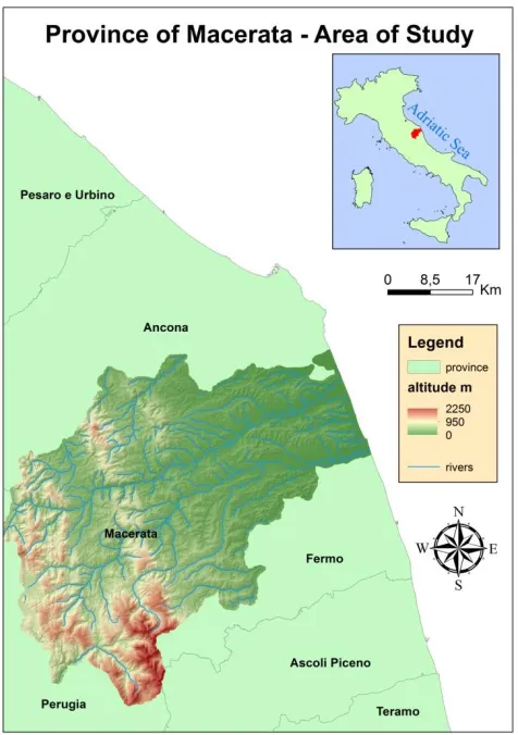
Macerata is the largest of the provinces in the Marche Region of Italy, with an area of about 2800
34
km2 (Figure 1). Macerata is bordered by the province of Perugia(Umbria Region) to the west, by the
35
Adriatic Sea, an arm of the Mediterranean Sea, to the east, and by three other provinces in the same
36
Region, Ancona to the north, Fermo to the south and Ascoli Piceno to the southwest.
37
38
Figure 1 - Geography of the study area.
39
This part of Central Italy is a transition point between coastal areas with a Mediterranean
40
climate, an inland Temperate climate and then to the west the Highland climates of the mountains
41
(Cs, Cf and H respectively in the Kӧppen-Geiger classification [1]). In some years there is a
42
dominance of one climate type over the other, even if this difference is only shown strongly in the
43
coastal zone. The aim of the present study was to create a new way to analyze temperature and
44
precipitation, through GIS software, in order to have a spatial analysis of climate variability across
45
this topographically complex region. In the literature there are several climate reports for Italy, but
46
not for the Marche Region. Indeed, there is only one published work, by the Experimental
47
Geophysical Observatory of Macerata [2] which can be considered a climate report. In this, an
48
arbitrary time interval from 1950 to 2000 is considered, which is not in line with the WMO (World
49
Meteorological Organization) approach [3]. There are two different studies for the Marche Region
50
focusing on climate change aspects. One considers the variations through projections until 2100
51
using climate modeling [4] and the other investigates the extreme indexes [5], to assess whether
52
there are any trends in the observed data. Finally there is another study for a larger area in Central
53
Italy that analyses climatic variations in relation to land, sea, social reaction and adaptation [6], but
54
this does not consider the Marche Region. Consequently, there is a lack of any detailed studies
55
analyzing and mapping temperature and precipitation patterns in Macerata province which can
56
highlight climate change.
57
2. Materials and Methods
58
Temperature and precipitation data were collected from 5 institutions: the former National
59
Hydrographic Service (SIMN), Multiple-Risk Functional Center of the Civil Protection, Italian Air
60
Force, Service Agency for the Agrifood Sector of the Marche Region (ASSAM), Functional Center of
61
obtained. For further analyses these were divided on the basis of 3 standard periods: 1931-1960,
63
1961-1990 and 1991-2014. The data were validated with 5 quality controls on the basis of the WMO
64
prescriptions [7] and through the procedures developed by Gentilucci et al. in 2018 [8]: logical and
65
gross error check, internal consistency check, tolerance test, temporal consistency, and spatial
66
consistency. For logical and gross error checking, temperatures outside the range (-40°C; +50°C)
67
were removed [9]and precipitation measurements greater than 2000 mm were also excluded [8]. The
68
internal consistency check verified the consistency of the data: for example, whether a maximum
69
value was higher than a minimum one, for temperature, and if there were negative values for
70
precipitation. Temporal consistency was useful to investigate errors between temporally contiguous
71
values, for example if there is too much difference between one day and the next, by setting a limit of
72
3 times the standard deviation added (upper limit) or subtracted (lower limit) to the mean [10]. In
73
the case of temporal consistency, the deletion of data is not immediate, but was subject to the spatial
74
consistency. The spatial consistency was performed taking into consideration the neighbouring
75
weather stations, grouped on the basis of their similarity [8]. After validation, climate data were
76
homogenized through the creation of a reference time series for each candidate weather station.
77
There are no reference weather stations of demonstrated reliability near the study area, so to assess
78
the suitability of the data it is necessary to reconstruct some reference time series to compare the
79
weather stations under investigation. The creation of the reference time series was performed daily
80
on the basis of 10 neighbouring weather stations, for all investigated periods, with empirical
81
Bayesian kriging (EBK), after a comparison with the inverse distance weighted (IDW) and the
82
ordinary co-kriging based on altitude, which is the most correlated independent variable [11]. An
83
interpolation was then prepared for each day by EBK and the climate value taken in the exact
84
coordinates of the weather station under investigation. The creation of the reference time series for
85
each weather station is indispensable for the analysis of breakpoints, which are points where there is
86
a sudden difference (an error) between the reading before and after the current one in the climatic
87
values time series of the same weather station. The breakpoints were analyzed through the SNHT
88
(Standard Normal Homogenity Test) [12], and the penalized t-test [13] was used to avoid an excess
89
of false breakpoints near the extremes of the time series. Finally, again using the SNHT method, the
90
time series was homogenized, multiplying it with the ratio between the mean before and after
91
shifting, produced by the breakpoint. The aim was to homogenize the time series of the weather
92
station with the most reliable part of it, which is mainly represented by the latest climate values (if
93
there are no systematic errors detected in the most recent data of the time series). A GIS database
94
was then prepared by editing a detailed Digital Elevation Model (DEM) with a cell size 5x5 m,
95
obtained using CTR (Regional Technical Map, Regione Marche, 2000), topographical map and
96
LIDAR reliefs [14]. The relationship of climatic variables with topographical parameters was
97
assessed and the elevation has been found to be the most correlated factor [15]. Thus, the DEM was
98
essential for data interpolation, in order to improve the results through the use of the geostatistical
99
technique of ordinary co-kriging, chosen after a cross-validation assessment between kriging
100
(ordinary and simple), empirical Bayesian kriging and Co-kriging (ordinary and simple). Co-kriging
101
was the method that minimized the error (in terms of Mean Error, RMSE, Mean Standardized error,
102
RMSSE, Mean standard error) more than all others, it was prepared with altitude as independent
103
variable and precipitation or temperature as the dependent one. The interpolation maps obtained
104
were compared between different periods (1931-1960, 1961-1990, 1991-2014) through GIS with the
105
mathematics between rasters, in order to assess spatial climatic variations.
106
3. Results
107
This section may be divided by subheadings. It should provide a concise and precise
108
description of the experimental results, their interpretation as well as the experimental conclusions
109
that can be drawn.
110
3.1. Data quality control
112
The first important result achieved was to have reliable data after the accurate quality controls
113
and homogeneity tests have been carried out. The validation process removed 0.02 % of the data for
114
temperature and 1.67 % of the data for precipitation. Instead, the homogenization, performed with
115
the SNHT and the Penalized T-test, after a long process of reference time series construction,
116
involved only the data of 4 weather stations. The EBK [16] was compared with IDW and ordinary
117
co-Kriging and was found that it improves the performance of IDW of about 5% (in terms of root
118
mean square error) on the same dataset, while it is quicker and easier, even if less accurate than
119
ordinary co-kriging (Table 1).
120
Table 1- Comparison between 3 interpolation methods (Inverse Distance Weighting (IDW),
121
empirical Bayesian kriging (EBK) and Ordinary Co-Kriging).
122
Statistical quality parameters IDW EBK Co-Kriging
Regression function 0.6x + 6.8 0.7x + 5.7 0.9x + 1.2
Mean 0.0119 0.0311 0.0566
Root-mean-square 1.6870 1.6429 1.2465
Mean standardized -0.0002 0.0237
Root-mean-square-standardized 0.9514 0.9890
Mean standard error 1.7366 1.5278
The reference time series obtained with EBK was related with the candidate time series, in order
123
to investigate if this series (candidate) needs homogenization. The result of subsequent
124
homogenization leads to 2 weather stations homogenized for temperature and 2 rain gauges for
125
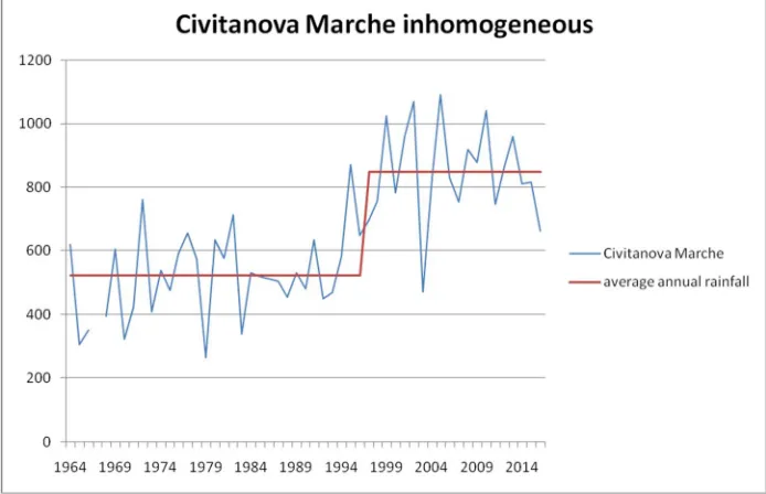
precipitation. In particular, the case of Civitanova Marche, a city on the Adriatic coast, is particularly
126
evident with a growing mean, after the breakpoint, of about 300 mm (Figure 2) which is
127
homogenized by the tests [12,13] (Figure 3).
128
129
Figure 2 - Civitanova Marche rain gauge inhomogeneous.
130
132
Figure 3 - Civitanova Marche rain gauge homogeneous.
133
3.2. Assessment of correlation between topographical and climatic variables
134
The adjusted data were used for the creation of detailed interpolation maps, passing through an
135
assessment of the influence of topographic co-variables on precipitation and temperature in this area
136
for all investigated periods (1931-1960/1961-1990/1991-2014). Six different topographic variables
137
were considered [11]: altitude, distance from the sea, latitude, distance from the closest river, aspect,
138
and distance from the crest line. The variables were assessed using the adjusted coefficient of
139
determination (R2) [11], with an assessment of the goodness of correlation represented by the
140
calculation of the standard error of the mean and the F-test. These 3 parameters can explain the
141
relation between the topographic variables and temperature or precipitation; in fact the R2 adjusted
142
(R2adj) shows the amount of variation explained by the estimated regression line (Figure 4) [17]:
143
= 1 − (1 − ) (1)
144
= sample size
145
= number of explanatory variables (independent), in this case 6
146
= ∑( ̅)( )
∑( ̅) ∑( ) (2)
147
148
̅ and = mean values of dependent and independent variables
149
and = values of dependent and independent variables
150
151
The standard error of the mean allows calculation of the dispersion of sample means around the
153
population, and also in this case the altitude shows the better value compared to the other
154
topographic variables both for temperature (Table 2) and precipitation (Table 3). Finally, the F-test
155
was performed to estimate if there can be a significant difference (based on 5% of rejection
156
probability) between the sample means of precipitation or temperature and those of the geographic
157
variables. When the variances of the two populations are equal, the variable cannot be used as
158
independent to obtain a correlation factor with the dependent one, because both of them would be
159
estimators of an unknown quantity σ2. The variance is an index of variability and it's expressed by
160
the formula:
161
162
=∑ ( ̅) (2)
163
whilst the F-test is obtained from the ratio between major and minor sampling variances.
164
= (3)
165
As demonstrated in Gentilucci et al., 2018 [11] for precipitation (Table 3), even for temperatures
166
the most correlated variable for the whole period (1931-2014) is the altitude (Table 2).
167
Table 2 - Comparison between topographic variables and mean annual temperature 1931-2014.
168
Regr. stats for T Alt.-yrs T 1931-2014 Dist. sea-yrs T 1931-2014 Lat.-yrs T 1931-2014 Dist. river-yrs T 1931-2014 Aspect-yrs T1931-2014 Dist. cre.-yrs T 1931-2014R2adj. 0.84 0.46 0.44 0.06 -0.01 -0.02
Std error 0.76 1.40 1.43 1.86 1.92 1.93
Sign. F 8.31 E-18 4.29 E-07 9.03 E-07 0.07 0.49 0.84
Table 3 - Comparison between topographic variables and mean annual precipitation 1931-2014.
169
Regr.stats for P Alt.-yrs P1931-2014 Dist. sea-yrs P 1931-2014 Lat.-yrs P 1931-2014 Dist.river-yrs P 1931-2014 Aspect-yrs P 1931-2014 Dist. cre.-yrs P 1931-2014R2adj. 0.70 0.69 0,26 0.07 -0.02 -0.02
Std error 102.32 103.50 159.80 178.40 187.33 187.39
Sign. F 6.92E-13 1.14E-12 2.24E-4 0.04 0.75 0.79
Thus, Tables 2 and 3 highlight the goodness of the correlation between altitude and
170
temperature or precipitation, in order to have a reliable independent variable for interpolation by
171
cokriging methods.
172
3.3. Interpolation and climate change analysis
173
Interpolation was performed by analysing three different types of cokriging, in order to identify
174
the most suitable for the available data:
175
Ordinary co-kriging, [18] a particular case of the universal cokriging, in which the residuals
176
mean is assumed constant and unknown.
177
( ) = ∑ ( ) ( ) +∑ ( ) ( ) (4)
178
( ) ( )= weights of the data assigned to and varies between
179
0 and 100%.
180
= regionalized data at a given location,primary and secondary data.
181
Simple co-kriging, [18] is used when the mean is stationary and the residuals mean is
182
considered a global constant and known in the whole study area, this method can be good only
183
if there are a large number of sample points.
184
( ) − = ∑ ( ) ( ) − +∑ ( ) ( ) + (5)
= mean of the primary and secondary data
186
Universal Co-Kriging, [19] a generalization of the ordinary cokriging, is used when the mean
187
isn't stationary, i.e. if there is a trend, and the residual isn't correlated to the trend (stationarity
188
of the residuals).
189
( ) = + + ∑ ( ) ( ) +∑ ( ) ( ) (6)
190
= mean of the residuals in the primary and secondary variable.
191
Ordinary cokriging has been chosen by an iterative process through many tests of
192
cross-validation performed within the ArcGis extension, Geostatistical Analyst. In the interpolations
193
the independent variable was elevation, whereas the dependent variable was temperature or
194
precipitation [20]. All interpolations were verified through 4 statistical indicators [21], which
195
allowed selection of the correct parameters for the semivariogram setting:
196
1. Root Mean Square Error (RMSE) - the standard deviation between observed and predicted
197
values: this parameter allows an assessment of the prediction errors for different weather
198
stations. However, RMSE isn't an absolute parameter, since it's impossible to compare different
199
variables with the RMSE; anyhow it can be anuseful to compare within the same data set. The
200
value of RMSE should be the smallest possible and similar to the ASE (mean standard error): in
201
this way when it is predicting a value in a point without observation points, it has only the ASE
202
to assess the uncertainty of the prediction.
203
∑ [ ( ) ( )]
(7)
204
( ) = measured value at position ;
205
( ) = predicted value at position ;
206
= number of weather stations;
207
=standard deviation of the population.
208
2. Mean Standard Error (ASE) - this statistical tool is known from the mean and it is used to
209
estimate the standard deviation of a sampling distribution. The ASE is an estimator of the bias
210
of the RMSE (i.e. the standard deviation of the estimation error). A value close to zero and
211
similar to RMSE represents a very low error in the estimation of the variability of the sampling
212
distribution.213
∑ ( ) (8)214
3. Mean Standardized Error (MSE) - It's similar to the mean error and calculates the difference
215
between measured and predicted values; however MSE values aren't related to single variables,
216
but it can be used to compare different variables. The standardization procedure leads a
217
variable with mean x and variance σ2, to another with mean zero and variance equal to 1, in
218
order to allow comparison between different variables. The mean standardized error is
219
represented by the ratio between the mean absolute error and the standard deviation of the
220
estimation error.221
∑ [ ( ) ( )]/ ( ) (9)222
4. Root Mean Square Standardized Error (RMSSE) - allows assessment of the goodness of
223
prediction models. It is desirable to have a value close to 1. If the value of RMSSE is lower than 1
224
the variability is overestimated, otherwise it is underestimated. This is a dimensionless
225
statistical tool, independent from the considered variable; it is the most significant instrument
226
to evaluate the interpolative model with other variables.
227
∑ [ ( ) ( )/ ( )]
(10)
228
The results of this cross-validation were represented by a table (for example Table 4) for each
229
interpolations for temperatures (maximum, mean, minimum) [22] and precipitation, on a monthly
231
and annual basis.
232
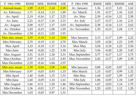
Table 4 - Period 1961-1990, statistical indicators for interpolations of maximum, mean and minimum
233
temperatures
234
P. 1961-1990 RMSE MSE RMSSE ASE P. 1961-1990 RMSE MSE RMSSE ASE Annual mean 1,89 -0,15 1,14 2,05 Av. January 1,36 -0,13 1,01 1,62 Av. February 1,71 -0,14 1,13 1,89 Av. March 1,91 -0,17 1,16 2,01
Av. April 2,19 -0,16 1,17 2,25 Av. May 2,39 -0,16 1,21 2,58
Av. June 2,21 -0,17 1,16 2,31 Av. July 2,17 -0,17 1,16 2,31 Av. August 2,00 -0,17 1,17 2,03 Av. September 2,38 -0,14 1,13 2,62 Av. October 1,83 -0,15 1,08 1,95 Av. November 1,55 -0,13 1,04 1,71 Av. December 1,54 -0,11 1,02 1,91
Max ann. mean 3,05 -0,18 1,14 3,04 Max January 2,15 -0,17 1,09 2,22 Max February 2,70 -0,19 1,12 2,70 Max March 3,05 -0,20 1,23 2,95
Max April 3,23 -0,18 1,17 3,16 Max May 3,54 -0,18 1,23 3,54
Max June 3,44 -0,20 1,22 3,30 Max July 3,56 -0,20 1,20 3,43
Max August 3,51 -0,19 1,18 3,31 Max September 3,77 -0,17 1,17 3,75 Max October 2,97 -0,19 1,12 2,83 Max November 2,42 -0,17 1,09 2,38 Max December 2,35 -0,16 1,04 2,57
Min ann. mean 1,30 -0,04 1,08 1,44 Min January 0,88 -0,05 0,87 1,18 Min February 0,97 -0,03 0,93 1,33 Min March 1,15 -0,07 0,99 1,32
Min April 1,40 -0,06 1,15 1,53 Min May 1,68 -0,07 1,09 1,87
Min June 1,60 -0,05 1,14 1,61 Min July 1,86 -0,05 1,18 1,69 Min August 1,66 0,11 1,20 1,46 Min September 1,67 -0,03 1,14 1,79 Min October 1,36 -0,01 1,17 1,41 Min November 1,20 -0,01 1,12 1,28 Min December 1,03 -0,05 0,97 1,31
The table (Table 3) highlights the quality of interpolation, with the statistical indicators always close
235
to the optimum value of the 4 statistical indicators. In fact, the value of the root mean square error
236
standardized is about 1 in all interpolations and the mean standardized error is close to 0. In this way
237
65 maps were created, in order to observe the distribution of temperature maximum, mean,
238
minimum and of precipitation, in the area of study. The varied climate condition of Macerata
239
Province is shown in (a)
240
(b)
241
Figure 5: there is a decrease of temperature and an increase of precipitation going from east
242
244
(a) (b)
245
Figure 5 - Mean annual temperature (a) and mean annual precipitation (b) in the period 1991-2014
246
for Macerata province.
247
The interpolation maps were averaged with the raster math tool, in order to compare different
248
periods of the same parameter. A positive trend from the past to the present is evident for
249
temperature, and a negative one for precipitation ( (a)
250
(b)
251
Figure 6).
252
253
(a) (b)
254
Figure 6 - Interpolation annual mean of the 3 periods (1931-1960/1961-1990/1991-2014) for
255
temperature (a) and precipitation (b).
256
Finally, the most important part of this research is represented by the comparison between the
257
interpolation maps of 1931-1960 and those of 1991-2014, to assess climate change in the last 60 years.
258
These variation maps (Figure 7) were obtained through the raster math tool, by subtracting to the
259
261
Figure 7- Variations of mean annual temperature between 1991-2014 and 1931-1960.
262
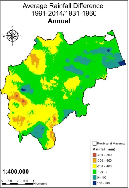
Figure 8 - Variations of mean annual rainfall between 1991-2014 and 1931-1960.
264
The variation map of mean temperature (Figure 7) shows a strong increase in the hilly zone, the
265
central part of the study area, while there is a slight decrease of temperature in the mountainous
266
region (west). For mean annual rainfall, the variation map (Figure 8) highlights a decrease in
267
precipitation over the whole province overall, but with small localized parts in which there is an
268
increase.
269
270
271
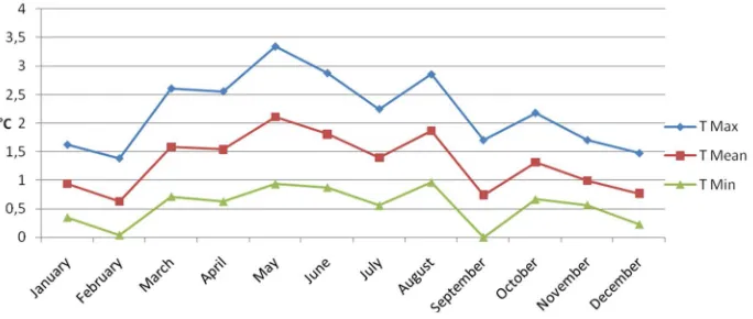
Figure 9 - Monthly temperature variations (maximum, mean and minimum) between the periods
272
1991-2014 and 1931-1960.
273
The graphs (Figure 9) records the differences on average in the whole territory between the
274
periods 1991-2014 and 1931-1960; it highlights, for each parameter, a bell-shaped trend strongly
275
increasing in spring and summer months, with a drop during winter and autumn. In February and
276
September, minimum temperatures are in a counter trend because there is no trend a strong
277
temperature increase in these two months.
278
279
Figure 10 - Trend of monthly variations in precipitation between the periods 1991-2014 and
280
1931-1960 for precipitations.
281
Precipitation has a reverse trend compared with temperatures (Figure 10) in that there is an
282
absence or even an augmentation of precipitation in spring and summer, while the decreasing peak
283
is focused on January, February and October, with significant amount between 25 mm and 35 mm.
284
December is an exception, because it shows the highest augmentation of rainfall (about 15 mm).
285
4. Discussion
286
This analysis has achieved some important goals for understanding and mapping the climate of
287
Macerata Province, Italy. Firstly, it has described the conditions of temperature and precipitation of
288
Macerata province in 3 different standard periods 1931-1960, 1961-1990, 1991-2014. The GIS software
289
precipitation. Furthermore, a strong relationship with altitude has been identified. In fact,there is a
291
differentiation that follows the altitudinal trend quite well, from the coast with high temperature,
292
even if the highest temperatures are located in the hilly belt behind the coast, to the lowest
293
temperatures in the Appennine Mountains (west). For precipitation, the smallest amount occurs on
294
the southern part of the coast, while the highest quantity is in the Appennine Mountains to the
295
south-west.
296
The second and most important result is represented by the study of climate change, with GIS
297
software in order to assess the variations through algebraic operations between rasters. The
298
differences between the period 1991-2014 and 1931-1960 were investigated in order to assess the
299
climatic change in the last 60 years. Generally, the amount of precipitation from 1931-1960 to
300
1991-2014 is diminished while the temperature is increased. However, spatially the situation is more
301
complex. In fact there is a central part of the study area in which temperature increased strongly by 2
302
to 3°C, while near the coast and in the mountains the change is about 0-1°C, with small decreases
303
focused in the Appennine and foothill belt (-1 to 0°C). For precipitation, the decrease is fairly
304
uniform across the study area (between about 0-200 mm), but with some isolated areas of strong
305
increase (200-300 mm) and only few parts of territory in which there is an increase of 0-200 mm,
306
mainly in the southern part of the coast, to the south-west and inland immediately behind the coast.
307
The monthly temperature trend is characterized by a constant growth, while for precipitation there
308
is a strong decrease in the amount measured in January, February and October (between 25 and 35
309
mm on average). This analysis, unlike previous studies, allows consideration of thespatial climate
310
change, which is moderately strong and unequivocal, but with some important counter-trends. In
311
future it would be interesting to investigate the variations between the different areas within the
312
province. Furthermore, to improve analysis, it would be desirable to install more reliable weather
313
stations, especially in the Appennine area (as this is under sampled).
314
Author Contributions: M.G., M.B., P.B. analyzed data; M.G. software GIS; M.G., M.B., P.B. wrote the paper;
315
M.G. Methodology, P.B. checked language.
316
Funding: This research received no external funding.
317
Conflicts of Interest: The authors declare no conflict of interest.
318
References
319
1. Köppen, W.; Geiger, R. Klima der Erde (Climate of the earth), 1954, Wall Map 1:16 Mill. Klett-Perthes,
320
Gotha.
321
2. Amici, M.; Spina, R. Campo medio della precipitazione annuale e stagionale sulle Marche per il periodo
322
1950-2000. Centro di Ecologia e Climatologia - Osservatorio Geofisico Sperimentale: Macerata, IT, 2002.
323
3. World Meteorological Organization (WMO), Handbook on CLIMAT and CLIMAT TEMP reporting.
324
WMO/TD No. 1188, Geneva, Switzerland, 2009.
325
4. Sangelantoni, L.; Coluccelli, A.; Russo, A. EGU General Assembly Conference Abstracts, 16, 1790, Wien,
326
2014.
327
5. Soldini, L.; Darvini, G. Extreme rainfall statistics in the Marche region, Italy. Hydrology Research 2017, 48(3),
328
686-700, nh.2017.091.
329
6. Appiotti, F.; Krželj, M.; Russo, A.; Ferretti, M.; Bastianini, M.; Marincioni, F. A multidisciplinary study on
330
the effects of climate change in the northern Adriatic Sea and the Marche region (central Italy). Reg Environ
331
Change, 2014, 14,(5), 2007-2024, https://doi.org/10.1007/s10113-013-0451-5.
332
7. World Meteorological Organization (WMO), Guidelines on Quality Control Procedures for Data from
333
Automatic Weather Stations. CBS/OPAG-IOS/ET AWS-3/Doc. 4(1), 2, Geneva, Switzerland, 2004.
334
8. Gentilucci, M.; Barbieri, M.; Burt, P.; D’Aprile, F. Preliminary Data Validation and Reconstruction of
335
Temperature and Precipitation in Central Italy. Geosciences 2018, 8 (6), 202, 10.20944.
336
9. Grykałowska, A.; Kowal, A.; Szmyrka-Grzebyk, A. The basics of calibration procedure and estimation of
337
uncertainty budget for meteorological temperature sensors. Met. Apps. 2015, 22, 867–872,10.1002.
338
10. Omar, M.H. Statistical Process Control Charts for Measuring and Monitoring Temporal Consistency of
339
11. Gentilucci, M.; Bisci, C.; Burt, P.; Fazzini, M.; Vaccaro, C. Interpolation of Rainfall Through Polynomial
341
Regression in the Marche Region (Central Italy). In: Mansourian A., Pilesjö P., Harrie L., van Lammeren R.
342
(eds) Geospatial Technologies for All AGILE 2018. Lecture Notes in Geoinformation and Cartography,
343
Springer, Cham, 2018, 55-73, https://doi.org/10.1007/978-3-319-78208-9_3.
344
12. Alexanderson, H.A. A homogeneity test applied to precipitation data. J. Climatol. 1986, 6, 661–675,
345
https://doi.org/10.1002/joc.3370060607.
346
13. Wang, X.L.; Wen, Q.H.; Wu, Y. Penalized Maximal t Test for Detecting Undocumented Mean Change in
347
Climate Data Series. J. Appl. Meteor. Climatol. 2007, 46, 916–931, https://doi.org/10.1175/JAM2504.1.
348
14. Liu, X.; Hu, H.; Hu, P. Accuracy assessment of lidar-derived digital elevation models based on
349
approximation theory. Remote Sensing 2015, 7(6), 7062-7079, 10.3390.
350
15. Diodato, N. The influence of topographic variables on the spatial variability of precipitation over small
351
regions of complex terrain. Int. J. .Climatol. 2005, 25, 351–363, https://doi.org/10.1002/joc.1131.
352
16. Krivoruchko, K. Empirical Bayesian Kriging, Esri, Redlands, CA, USA, 2012.
353
17. Witt, G. Using Data from Climate Science to Teach Introductory Statistics, J. Stat. Educ. 2013, 21, 1,
354
https://doi.org/10.1080/10691898.2013.11889667.
355
18. Goovaerts, P., Ordinary Cokriging Revisited. Math. Geol. 1998, 30, 1, 21-42,
356
https://doi.org/10.1023/A:1021757104135.
357
19. Helterbrand, J.D.; Cressie, N. Universal cokriging under intrinsic coregionalization, Math. Geol. 1994, 26,
358
205. https://doi.org/10.1007/BF02082764.
359
20. Newlands, N. K.; Davidson, A.; Howard, A.; Hill, H. Validation and inter-comparison of three
360
methodologies for interpolating daily precipitation and temperature across Canada. Environmetrics 2011,
361
22, 205–223. doi:10.1002/env.1044.
362
21. Johnston, K.; Ver Hoef, J. M.; Krivoruchko, K.; Lucas, N. Using ArcGIS geostatistical analyst, 380, Esri,
363
Redlands, CA, USA, 2001.
364
22. Ishida, T.; Kawashima, S.; Use cokriging to estimate surface air temperature from elevation. Theor. Appl.
365