https://doi.org/10.5194/amt-11-1971-2018 © Author(s) 2018. This work is distributed under the Creative Commons Attribution 4.0 License.
Intercomparison of middle-atmospheric wind in observations
and models
Rolf Rüfenacht1,a,b, Gerd Baumgarten1, Jens Hildebrand1, Franziska Schranz2, Vivien Matthias1, Gunter Stober1, Franz-Josef Lübken1, and Niklaus Kämpfer2
1Leibniz-Institute of Atmospheric Physics at the Rostock University, Kühlungsborn, Germany 2Institute of Applied Physics, University of Bern, Bern, Switzerland
anow at: Federal Office of Meteorology and Climatology MeteoSwiss, Payerne, Switzerland bnow at: Institute of Applied Physics, University of Bern, Bern, Switzerland
Correspondence:Rolf Rüfenacht ([email protected]) Received: 29 October 2017 – Discussion started: 21 November 2017
Revised: 23 February 2018 – Accepted: 7 March 2018 – Published: 6 April 2018
Abstract.Wind profile information throughout the entire up-per stratosphere and lower mesosphere (USLM) is impor-tant for the understanding of atmospheric dynamics but be-came available only recently, thanks to developments in re-mote sensing techniques and modelling approaches. How-ever, as wind measurements from these altitudes are rare, such products have generally not yet been validated with (other) observations. This paper presents the first long-term intercomparison of wind observations in the USLM by co-located microwave radiometer and lidar instruments at An-denes, Norway (69.3◦N, 16.0◦E). Good correspondence has
been found at all altitudes for both horizontal wind compo-nents for nighttime as well as daylight conditions. Biases are mostly within the random errors and do not exceed 5– 10 m s−1, which is less than 10 % of the typically encoun-tered wind speeds. Moreover, comparisons of the observa-tions with the major reanalyses and models covering this altitude range are shown, in particular with the recently re-leased ERA5, ECMWF’s first reanalysis to cover the whole USLM region. The agreement between models and observa-tions is very good in general, but temporally limited occur-rences of pronounced discrepancies (up to 40 m s−1) exist. In the article’s Appendix the possibility of obtaining nighttime wind information about the mesopause region by means of microwave radiometry is investigated.
1 Introduction
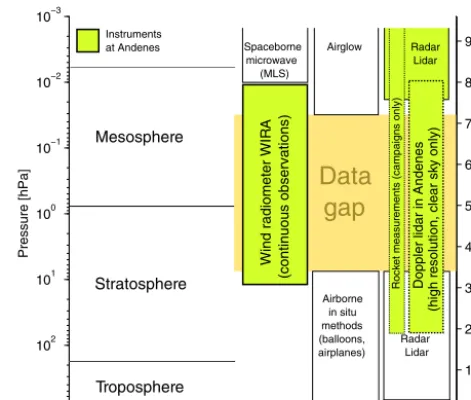
Measurements of the wind field in the upper stratosphere and lower mesosphere (USLM) are challenging. The con-sequence is a substantial data gap between 10 and 0.03 hPa (∼32 to 70 km). Figure 1 summarises the altitude coverage of the currently existing wind measurement techniques.
The widely used radar techniques can usually not assess the USLM due to the lack of backscatterers (charged parti-cles, turbulent structures at scales of the radar wavelength). Only in the event of strong particle precipitations have mea-surements down to 60 km been reported (e.g. Nicolls et al., 2010; Shibuya et al., 2017; for an encompassing overview on radar observation techniques refer to e.g. Hocking, 2016). At the same time, the transport of in situ sensors to these alti-tudes cannot be achieved with radiosoundings or airplanes. For many years rocket-aided measurements were thus the only way to overcome this data gap. Such observations have been carried out since the 1960s (National Research Coun-cil, 1966). They offer high vertical resolution but are very manpower and cost intensive. Hence, measurements are only made on campaign basis so that the data set consists of snap-shots of the atmosphere highly scattered in time.
on nighttime stratospheric wind measurements by lidar (Chanin et al., 1989; Souprayen et al., 1999; Tepley, 1994; Friedman et al., 1997). Due to the novelty of the two ap-proaches and the absence of satellite data, thorough vali-dations with two independent measurement techniques syn-chronously assessing the same atmospheric volume are at a very early stage. Such intercomparisons at multi-instrument sites are a key activity of the Horizon 2020 project ARISE1 (Blanc et al., 2018). Previously, Lübken et al. (2016) pre-sented comparisons between observations with the ALO-MAR Rayleigh–Mie–Raman (RMR) lidar and eight night-time starute2soundings by rockets. In most cases good corre-spondence between both techniques has been found, even in the small-scale structures. However, for some soundings the intercomparisons suffered from differing spatial sampling. Such sampling issues are closely related to the snapshot na-ture of rocket measurements. They can largely be overcome when comparing techniques which allow longer observa-tion times, as it is the case for the radiometry and lidar ap-proaches, because atmospheric inhomogeneities tend to av-erage out over time. The RMR wind lidar and the ground-based wind radiometer WIRA have been operated next to each other at ALOMAR observatory in Andenes, Norway (69.3◦N, 16.0◦E), for a 11-month intercomparison period between 1 August 2016 and 30 June 2017. During this pe-riod, 518 h of coincident measurements of sufficient dura-tion3and an uninterrupted series of 187 h of continuous day and night observations have been recorded.
In parallel to the development of new measurement tech-niques most important general circulation models for numer-ical weather prediction and reanalysis have extended their lids further into the middle atmosphere due to the broad evidence for the influence of middle-atmospheric dynam-ics on tropospheric weather and climate (e.g. Baldwin and Dunkerton, 2001; Scaife et al., 2008; Kidston et al., 2015; Garfinkel et al., 2017). The most recent example of this trend towards increased model tops is the European Centre for Medium-Range Weather Forecast (ECMWF) ERA5 reanaly-sis released in July 2017, which extends up to 0.1 hPa, one pressure decade higher than its predecessor ERA-Interim. In addition to the improvement of the tropospheric forecast skills of the weather predictions, the higher model lids made available reanalysis data for the stratosphere and mesosphere which are widely used in the research community. However, up to now, only few comparisons between wind observations
1http://arise-project.eu.
2Stable retardation parachute, i.e. an extra-stable falling target
deployed by the rocket and tracked by ground-based radars (e.g. Schmidlin et al., 1985).
3Only measurements longer than 5 h are considered in this study
in order to mitigate effects of the different pointing of the instru-ments (see Sect. 4) and to guarantee stable radiometer retrievals.
0 10 20 30 40 50 60 70 80 90
Approx. altitude [km]
10−3
10−2
10−1
100
101
102
103
Pressure [hPa]
Mesosphere
Stratosphere
Troposphere
Data
gap
Radar Lidar Radar
Lidar Airglow
wind measurements
Sodar Airborne
in situ methods (balloons, airplanes) Spaceborne microwave
(MLS)
Dopple
r lida
r in Andenes
(high r
esolution, cle
a
r sk
y only)
Ro
c
k
e
t
m
e
a
s
u
re
m
e
n
ts
(
c
a
m
p
a
ig
n
s
o
n
ly
)
Wi
n
d
r
a
d
io
m
e
te
r
W
IR
A
(continuous
observations
)
Instruments at Andenes
Figure 1.Overview of the altitude coverage of the currently op-erational wind measurement techniques. The techniques available
at Andenes (69.3◦N, 16.0◦E), the observation site of the present
study, are highlighted.
and models exist4: Kishore Kumar et al. (2015) analysed the correspondence of fortnightly rocket wind soundings with the Modern-Era Retrospective analysis for Research and Applications (MERRA) reanalysis and Hildebrand et al. (2012, 2017) showed comparisons between January night-time lidar measurements and ECMWF operational analy-sis and forecast data. The present study will show for the first long-term intercomparisons between wind observations and state-of-the-art models and reanalyses (ERA5, ECMWF forecasts, MERRA2, SD-WACCM) by using the 11-month quasi-continuous data set recorded by the microwave ra-diometer WIRA.
In this paper the first part describes the measurement tech-niques for wind observations in the USLM (Sect. 2), the models and reanalyses used in this study (Sect. 3) and con-siderations to the effects of spatial and temporal sampling (Sect. 4). In Sect. 5 the intercomparisons between the coinci-dent lidar and radiometer observations are presented along-side the short-term comparisons to models. Model valida-tions on longer timescales are described in Sect. 6 before we draw the conclusions of our research in Sect. 7.
2 Measurement techniques
Figure 1 illustrates the unique situation of Andenes, Norway (69.3◦N, 16.0◦E), where all currently available wind mea-surement techniques covering the gap region in the USLM are concentrated. Wind radiometer, lidar and meteor radar are
4Le Pichon et al. (2015) noted that also middle-atmospheric
all contributing to the aforementioned ARISE project (Blanc et al., 2018).
2.1 Doppler microwave radiometry
Microwave radiation is emitted in transitions between rota-tional quantum levels of molecules with electric (or mag-netic) dipole moment, which are present in the gap region for wind observations in the USLM. Ground-based microwave radiometers have been widely used to determine the concen-trations of the emitting molecules, e.g. water vapour, ozone or carbon monoxide (Lobsiger, 1987; Nedoluha et al., 1995; Forkman et al., 2003; Palm et al., 2010; Fernandez et al., 2016). Technical developments, especially in the field of high-frequency low-noise amplifiers and spectrometer sta-bility/resolution, now enable the determination of the wind-induced Doppler shift of these emission signals. Altitude-dependent information is retrieved thanks to the pressure broadened nature of the emission spectra.
First measurements of profiles of horizontal wind by ground-based microwave radiometry had been presented by Rüfenacht et al. (2012). Recently, another similar instrument became operational and is currently set up at Maïdo ob-servatory on La Réunion island (Hagen, 2015). The possi-bility for spaceborne wind observations with a comparable approach has also been demonstrated: SMILES was oper-ated during 7 months onboard the International Space Sta-tion (ISS; Baron et al., 2013) and an early-stage project for a satellite microwave limb sounding wind instrument exists (Baron et al., 2015).
The ground-based Doppler microwave wind radiometer WIRA, which contributes to the present study, is an up-graded version of the instrument presented in Rüfenacht et al. (2012). For the determination of wind profiles the Doppler shifts of signals from opposite azimuths in 68◦off-zenith di-rection are compared. The retrieval algorithm which is based on the optimal estimation method (Rodgers, 2000) is sim-ilar to the version in Rüfenacht et al. (2014) with a con-stant zero wind a priori profile. In this study we use iden-tical a priori standard deviations for both horizontal wind components equivalent to 4 times the standard deviation of 6 years of zonal wind data from ECMWF. In order to account for the high nighttime ozone concentrations which occur in the mesopause region the retrieval algorithm has been im-proved according to Rüfenacht and Kämpfer (2017). It now uses distinct ozone a priori profiles for nighttime or sunlit periods at the mesopause, discriminated by the sunrise and sunset at 100 km altitude. Based on considerations to atmo-spheric physics and chemistry and radiative transfer as well as on the comparisons of the day–night differences in the radiometer observations and models presented in Rüfenacht and Kämpfer (2017) the authors judge now also the nighttime observations of mesospheric wind by WIRA to be largely bias-free. This quality is intended to be confirmed by the
first instrumental intercomparisons carried out in the present study.
The wind radiometer WIRA can provide zonal and merid-ional wind profiles with a vertical resolution of 10–16 km with minimal integration times of around 5 h. The trustwor-thy altitude range, i.e. where the measurement response is >0.8, the altitude resolution is<20 km and the altitude ac-curacy is<4 km (for details see Rüfenacht et al., 2014), typi-cally extends from 7 to 0.03 hPa (∼35 to 70 km). Microwave radiometers can be highly automatised and have the ability to pursue the measurements during overcast conditions what leads to near-continuous time series of observations, a char-acteristic that will be exploited for the model validations dur-ing almost a full annual cycle presented in Sect. 6.
2.2 Middle-atmospheric wind lidar
Lidar systems with powerful lasers, large telescopes and sensitive detection optics are able to get usable molecular backscatter from altitudes up to 70 to 80 km. When high fre-quency stability and calibration standards are met, wind can be determined from the Doppler shift of the backscattered signal. This is achieved by relating the recordings of a chan-nel containing elements with frequency-dependent transmis-sion in its receiver optics with recordings of a reference chan-nel without such elements.
The first observations of zonal and meridional wind by lidars covering the entire gap region in the USLM have been presented by (Baumgarten, 2010) using the RMR li-dar at ALOMAR, the instrument which is contributing to the present study. Validations of the method for nighttime ob-servations have been presented by Hildebrand et al. (2012) and Lübken et al. (2016). Measurements of temperatures and wind during day and night are presented in Baumgarten et al. (2015). Recently, middle-atmospheric wind measurements from a similar instrument have been reported by Yan et al. (2017).
The ALOMAR RMR lidar obtains wind information by single-edge iodine absorption spectroscopy on the 532 nm signal from 20◦ off-zenith. Injection-seeding of the trans-mitting lasers by a highly frequency-stable continuous wave laser, real-time monitoring of the wavelength transmitted to the atmosphere as well as regular calibrations of the fre-quency dependence of the transmission through the receiver optics and the iodine vapour cell assure the accuracy of the wind observations. Moreover, the exactitude of the calibra-tion is optimised by performing 1 h of vertical wind observa-tions at the beginning of each measurement run (for details see Baumgarten, 2010; Hildebrand et al., 2012).
sunrise at 16 km). The frequency-dependent optical proper-ties of the etalon and its effect on the different beam paths need to be accurately known from calibration measurements, what increases the complexity of the daylight wind mea-surements. In the previous rocket–lidar intercomparisons by Lübken et al. (2016) only nighttime wind profiles have been investigated. Daylight profiles will for the first time be vali-dated in the present study.
The ALOMAR RMR lidar delivers wind profiles with very high vertical and temporal resolution (natively 150 m and 5 min). Some binning of the data is usually applied for increasing the signal-to-noise ratio. The measurement un-certainty depends on altitude and ranges from about 1 to 10 m s−1at altitudes between 50 and 80 km for integration times of 1 h and vertical resolutions of 2 km. As for any middle-atmospheric lidar, the operation of the RMR lidar is limited to clear-sky conditions.
2.3 Meteor radar
Measurements from the Andenes meteor radar will be used in the present study although it is not directly covering the gap region for wind observations in the USLM. Indeed, the lowest altitudes covered by the meteor radar are adjacent to the uppermost levels covered by WIRA and the RMR lidar, at least in good observation conditions (reasonably low tro-pospheric water content for the radiometer, no cirrus clouds for the lidar). Hence, the meteor radar can help in the inter-pretation of the wind data at the highest levels of the USLM gap region.
Meteor radars providing wind observations through the evaluation of the drift of meteor trails in the wind field of the mesosphere–lower thermosphere region are a well-established technique (Hocking et al., 2001a; Jacobi, 2011; Fritts et al., 2012; Iimura et al., 2015). The reliability has also been demonstrated in recent comparisons to other re-mote sensing techniques and the Navy Global Environmen-tal Model (NAVGEM) (Reid, 2015; McCormack et al., 2017; Wilhelm et al., 2017).
The Andenes meteor radar operates at 32.55 MHz with a peak power of 30 kW. The typical altitude range extends from 75 to 105 km. Details of the retrieval algorithm have been presented in Stober et al. (2017).
3 General circulation models, reanalyses and geostrophic wind
3.1 ECMWF ERA5 and forecast data
The recently released ERA5 reanalysis (Hersbach and Dee, 2016) is the ECMWF’s first reanalysis to extend throughout the mesosphere up to 0.1 hPa. It provides hourly output so that a good temporal match with the observation data can be achieved. At the time of writing only the data prior to 31 December 2016 had been released. Therefore, alongside the
ERA5 high-resolution (HRES) data, hourly forecasts (FC) from IFS cycles 41r2 (from 1 August 2016 to 21 November 2016), i.e. the same cycle as for the ERA5 reanalysis, and 43r1 (from 22 November 2016 to 30 June 2017) are used in the present study (ECMWF, 2017a). ECMWF models and re-analyses use a 4DVAR assimilation scheme. The only source of upper-air assimilations are infrared nadir sounders (AIRS, HIRS, IASI; Dragani and McNally, 2013).
3.2 MERRA2
MERRA2 is the current reanalysis of NASA’s Goddard Earth Observing System-5 (GEOS-5) model with 3-hourly output extending up to 0.01 hPa (Molod et al., 2015). It is the succes-sor of the discontinued MERRA reanalysis used in the inter-comparison study by Kishore Kumar et al. (2015). In contrast to ECMWF’s models and reanalyses, MERRA2 also assimi-lates USLM observations from the Microwave Limb Sounder (MLS) on the Aura satellite (Waters et al., 2006) in a 3DVAR assimilation scheme. A detailed description of the MERRA2 reanalysis was recently presented by Gelaro et al. (2017). 3.3 SD-WACCM
Thanks to its model top as high as 6×10⁻⁶hPa, the Whole Atmosphere Community Climate Model (WACCM; Marsh et al., 2013) is a well-established data source for studies of middle-atmospheric dynamics. WACCM has a specified dy-namics version named SD-WACCM (Lamarque et al., 2012; Kunz et al., 2011) which is suitable for intercomparisons with measurements. To constrain the dynamics of the model, its temperature, horizontal wind and surface pressure fields are nudged with meteorological analysis data at every inter-nal time step. For the present study SD-WACCM was nudged to the GEOS-5 meteorological analysis data at each 30 min time step. The nudging coefficient is 10 %, which means that the nudged fields are defined as a linear combination of 90 % from the model and 10 % from GEOS5 data (Brakebusch et al., 2013). This nudging is performed up to 50 km, then it linearly decreases in strength to zero nudging above 60 km. In the model gravity waves are parameterised, whereas plan-etary waves are resolved (Richter et al., 2010). SD-WACCM has a free-running chemistry in the whole atmosphere. 3.4 Geostrophic wind from the MLS geopotential
height field
this approach has a very direct connection between the wind field and observed data at the altitudes of interest.
Here, we calculate the geostrophic zonal (ug) and
merid-ional (vg) wind from geopotential height (GPH) profiles of
MLS on board the Aura Satellite (Waters et al., 2006; Livesey et al., 2015) by
ug= −
1 f
∂8
∂y vg=
1 f
∂8
∂x, (1)
where 8 is the geopotential, f is the Coriolis parame-ter, and x andy are used to denote the partial derivatives (acosφ)−1∂λ∂ anda−1 1∂φ, whereλis longitude,φis latitude andais Earth’s radius. Note that in this formulation friction, vertical advection and time tendency is neglected and that the geostrophic balance is assumed, i.e. the exact balance between Coriolis force and pressure gradient force. There-fore the geostrophic wind is directed parallel to the isobars and does not depend on curvature at all, meaning that the air does not flow from high to low pressure. However, outside the tropics geostrophic wind can often be regarded as a rea-sonable approximation of the real wind.
MLS has a global coverage from 82◦S to 82◦N on each orbit and a usable height range from 261 to 0.001 hPa (11 to 97 km), with a vertical resolution of∼4 km in the strato-sphere and ∼14 km at the mesopause. Daily averages of version 4 MLS data were used and the most recent recom-mended quality screening procedures of Livesey et al. (2015) have been applied.
The GPH observations have a precision between ±30 m at the tropopause and±110 m at the mesopause level and a bias of 50 to 150 m in the troposphere and stratosphere and up to−450 m at 0.001 hPa (Froidevaux et al., 2006; Schwartz et al., 2008).
For the geostrophic wind estimation the original orbital MLS data are accumulated in grid boxes with 20◦grid spac-ing in longitude and 5◦in latitude and averaged over 1 day. This global smoothed data are then used to calculate the global geostrophic wind using Eq. 1. For the comparison with the local measurements the average geostrophic wind in the area 67–72◦N and 0–30◦E is chosen from the global calculations.
Some marginal aliasing effects on MLS data from the mi-grating tides cannot be excluded. However, since Aura is in a sun synchronous orbit, its samples are stationary with respect to migrating tides. These should appear as constant offsets to the measurements at a particular latitude. Especially the ef-fect of the diurnal tide, which appears to be the strongest tidal component in the middle atmosphere, is strongly re-duced by the averaging over the measurements during the satellite’s overpasses in the ascending and descending orbit spaced by 12 h. A more detailed discussion on the impact of tides on MLS measurements can be found for example in Lieberman et al. (2015) and Xu et al. (2009). It should also be remembered that, in contrast to the mesopause region, tides
are usually weak in the stratosphere and lower mesosphere (e.g. Baumgarten et al., 2018; Kopp et al., 2015; Sakazaki et al., 2018).
4 Spatial and temporal sampling of observations and models
A crucial aspect of intercomparisons of atmospheric data is to account for the different temporal and spatial sampling of the used instruments and models. Radiometer winds are re-trieved on pressure levels while the lidar operates on a ge-ometrical height grid; therefore all data are transformed to pressure coordinates according to the CIRA86 climatology (Fleming et al., 1990) for the respective day.
4.1 Horizontal and temporal sampling
The lidar observations are almost true point measurements; no horizontal averaging is involved. Due to their off-zenith nature the measured wind profiles are not completely verti-cal, e.g. the return signal at 70 km altitude originates from a point with a horizontal distance of 25 km to the observa-tory. Such small horizontal distances can safely be neglected in the present context. In contrast, the wind speeds obtained by the microwave radiometer involve measurements at two points horizontally distant by 2z·tan(68◦), wherezis altitude above the observatory, i.e. 150, 250 and 350 km at altitudes of 30, 50 and 70 km, respectively. The Andenes meteor radar obtains most meteor echoes from zenith angles between 50 and 60◦, leading to an average observation volume extent of about 160 km at an altitude of 70 km. Models and reanalyses also feature substantial horizontal smoothing so that particu-larly localised features are not captured. The data set with the lowest horizontal and temporal resolution are the geostrophic winds calculated from MLS GPHs (see Sect. 3.4).
4.2 Vertical sampling
In contrast to horizontal smoothing the vertical structures are far more persistent in time. Therefore it is important to con-sider the limited vertical resolution of microwave radiome-ters, which is on the order of 10–16 km for WIRA’s wind observations. To compare high-resolution data xi (where i
stands for lidar or model data) to the observations from WIRA, these should be convolved with the radiometer’s av-eraging kernels A(for details see Rüfenacht and Kämpfer, 2017) according to
xi,c=A(xi−xa)+xa, (2)
where the a priori wind profilexaused by the radiometer is
constantly zero. In the case of perfect instruments and mod-els, all profiles xi,c and the observations by WIRA would
agree within their random errors.
5 Intercomparisons for lidar operation times
In the sake of conciseness we mainly present averages over several days of measurements in this section. For the inter-ested reader the wind profiles from the radiometer, the lidar and the models for each individual day and night of observa-tion are reprinted in the Figs. S1 to S4.
The longest uninterrupted lidar measurement of the inter-comparison campaign took place from 3 to 11 February 2017 and lasted for 187 h. The time series of the lidar and radiome-ter zonal and meridional wind profiles are shown in Figs. 2 and 3, respectively.
These observations cover a particularly dynamic time pe-riod in the vicinity of a minor sudden stratospheric warming. For instance the zonal wind reverts its direction from−40 to 40 m s−1within a few days. Obviously the lidar time series feature structures of atmospheric waves which cannot be re-solved by the microwave radiometer. Beyond this difference of resolution the time series from the two instruments corre-spond very well.
In Fig. 2 the strong westward winds on 3 February, the pro-nounced decrease in the wind velocities at stratopause level in the evening of 4 February along with the wind direction being inverted to eastward above 0.3 and below 3 hPa are all captured by both instruments. The same is true for the fol-lowing westward acceleration on 5 and 6 February as well as the inversion of wind direction to eastward with two distinct wind speed maxima in the night of 8/9 and 10/11 February. It should be noted that also the altitudes and the timing of the features correspond very well. The most notable difference is that the radiometer wind at stratopause level on 4 Febru-ary stays slightly negative whereas the lidar reaches a zero zonal wind situation, which can mostly be attributed to the temporal averaging by WIRA that includes negative winds from before and after this event.
04 Feb 05 Feb 06 Feb 07 Feb 08 Feb 09 Feb 10 Feb 11 Feb 10-2
10-1
100
101
Pressure [hPa]
Zonal wind RMR lidar
-150 -100 -50 0 50 100 150
W
in
d
s
p
e
e
d
[
m
s
-1]
04 Feb 05 Feb 06 Feb 07 Feb 08 Feb 09 Feb 10 Feb 11 Feb 10-2
10-1
100
101
Pressure [hPa]
Zonal wind WIRA
-150 -100 -50 0 50 100 150
W
in
d
s
p
e
e
d
[
m
s
-1]
Figure 2.Time series of zonal wind during 187.1 h of coincident li-dar and radiometer measurements recorded at Andenes from 3 to 11 February 2017. For better visibility the lidar data are binned to 1 km vertical resolution while the temporal resolution is 5 min. The trust-worthy altitude range of the wind radiometer data, according to the definition given in Sect. 2.1, is marked by the horizontal dark grey lines. Data outside this range should not be considered as they may substantially be affected by a priori assumptions. All times are ex-pressed in coordinated universal time (UTC) with the ticks at 00:00.
04 Feb 05 Feb 06 Feb 07 Feb 08 Feb 09 Feb 10 Feb 11 Feb 10-2
10-1
100
101
Pressure [hPa]
Meridional wind RMR lidar
-100 -50 0 50 100
W
in
d
s
p
e
e
d
[
m
s
-1]
04 Feb 05 Feb 06 Feb 07 Feb 08 Feb 09 Feb 10 Feb 11 Feb 10-2
10-1
100
101
Pressure [hPa]
Meridional wind WIRA
-100 -50 0 50 100
W
in
d
s
p
e
e
d
[
m
s
-1]
Figure 3.As Fig. 2 but for the meridional wind component.
Wind speed [m s-1]
Pressure [hPa] Altitude [km]
0 20 40
Daylight meridional wind
62.5 h of measurements between 03 and 10 Feb 2017
radiometer lidar ECMWF FC MERRA2 SD-WACCM geostrophic meteor radar
-20 -10 0 10
10-2
10-1
100
101
Daylight zonal wind
62.5 h measurements between 03 and 10 Feb 2017
Radiometer Lidar ECMWF FC MERRA2 SD-WACCM Geostrophic Meteor radar
35 40 45 50 55 60 65 70 75 80
Figure 4.Mean daytime zonal and meridional wind profiles for the observation period 3–11 February 2017 measured by the wind ra-diometer WIRA and the RMR lidar in comparison with models, re-analyses and geostrophic wind calculations from MLS geopotential heights. All middle-atmospheric comparison data have been con-volved with WIRA’s averaging kernels according to Eq. (2) and cut at the limits of the trustworthy altitude range of the coincident ra-diometer observation. The discontinuities in the profiles visible at the uppermost altitudes originate from the averaging over obser-vations with slightly different altitude coverage. At the uppermost altitudes the simultaneous observations from the meteor radar (not convolved) are shown. The random errors of all measurement data are denoted by dotted lines. Only data from times when lidar and ra-diometer were both operated in their respective daylight mode have been considered in this plot.
For more quantitative analyses the average daylight and nighttime wind profiles of this measurement period are pre-sented in Figs. 4 and 5, respectively. The wind at each level has been averaged with the weights being the integration times1ti of data sampled at this level during measurement i, i.e. uavg=P(1ti·ui)/P1ti. The errors of these
aver-age winds were accordingly calculated using Gaussian error propagation:σavg=pP(1ti·σi)2/P1ti.
Generally daylight observations are more challenging for the lidar because of potential uncertainties related to the po-sitioning of the additional Fabry–Pérot Etalon, whereas the nighttime radiometer wind measurements were known to be biased before the upgrade of the retrieval by Rüfenacht and Kämpfer (2017). Only time periods when lidar and radiome-ter are both in their respective daylight or nighttime config-urations have been considered in the following analyses in order to independently validate both modes of each instru-ment.
For the daylight periods (Fig. 4) both observations and all models are in very close agreement at all altitudes and for both wind components. They all lie well within the random errors, which are more than 1 order of magnitude smaller than the fluctuations of the atmospheric wind during this
Wind speed [m s-1]
Pressure [hPa] Altitude [km]
0 20 40
Nighttime meridional wind
104.2 h of measurements between 03 and 11 Feb 2017
radiometer lidar ECMWF FC MERRA2 SD-WACCM geostrophic meteor radar
-20 0 20
10-2
10-1
100
101
Nighttime zonal wind
104.2 h of measurements between 03 and 11 Feb 2017
Radiometer Lidar ECMWF FC MERRA2 SD-WACCM Geostrophic Meteor radar
35 40 45 50 55 60 65 70 75 80
Figure 5.As Fig. 4 but for data from the time period when both instruments were operated in their respective night mode.
time. Only the meridional component of the geostrophic wind calculations shows an offset. This is, however, not sur-prising when considering the coarse resolution of this data set in combination with a very dynamic period with pronounced wind gradients around Andenes.
During nighttime (Fig. 5), up to 0.3 hPa, all data sources agree within WIRA’s observation errors or are very close. Above, substantial differences among the various data sources are visible. Notably the radiometer and lidar zonal winds agree throughout the entire altitude range and the ECMWF forecasts are close to the observations. In contrast, MERRA2 is slightly offset by 7 m s−1 and SD-WACCM
Difference to radiometer wind speed [m s-1]
Pressure [hPa] Altitude [km]
-20 -10 0 10 20
Daylight meridional wind
325.5 h of measurements between 04 Aug 2016 and 24 Jun 2017
lidar ECMWF FC MERRA2 SD-WACCM geostrophic
-20 -10 0 10 20
10-2
10-1
100
101
Daylight zonal wind
348.2 h of measurements between 04 Aug 2016 and 24 Jun 2017
Lidar ECMWF FC MERRA2 SD-WACCM Geostrophic
35 40 45 50 55 60 65 70 75 80
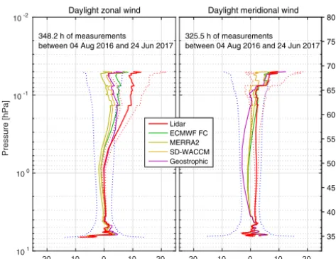
Figure 6. Mean difference of all convolved daytime zonal and meridional wind profiles from models, reanalyses, MLS geostrophic winds and the RMR lidar to the observations from WIRA recorded during the entire intercomparison campaign. The bands of random errors of the radiometer and the lidar observations are denoted by blue and red dotted lines, respectively. The discon-tinuities in the profiles visible at the upper and lowermost altitudes originate from the averaging over observations with different alti-tude coverage. Only data from the time period when both instru-ments were operated in their respective daylight mode have been considered.
microwave emissions. In any case, as the zonal wind mea-surements are in very close agreement it is not believed that the high-altitude differences in meridional wind observations during these times indicate a fundamental instrumental prob-lem.
The mean differences to the wind radiometer profiles over all measurements made during the entire 11-month intercom-parison campaign are shown in Figs. 6 and 7.
In total 348 and 326 h of coincident daylight as well as 169 and 158 h of nighttime zonal and meridional wind obser-vations meeting the >5 h criterion have been made by the lidar and the radiometer, respectively. The slightly reduced measurement time for the meridional component is due to the downtime of one power laser caused by its flash lamps reaching the end of their life cycle in October 2016. For an overview of the temporal distribution of lidar observations along with the dynamical situation around these recordings, the interested reader is referred to Figs. 9 and 10 in Sect. 6, where days with lidar measurements are marked by green dots.
The daylight zonal winds of all models agree within the radiometer’s random errors (Fig. 6). The lidar and the ra-diometer are in close correspondence up to 0.3 hPa, above the lidar has recorded more eastward winds with offsets of up to 10 m s−1also slightly disagreeing with the models. One should, however, note the increasing uncertainty at these
al-Difference to radiometer wind speed [m s-1]
Pressure [hPa] Altitude [km]
-20 -10 0 10 20
Nighttime meridional wind
158.1 h of measurements between 20 Sep 2016 and 11 Feb 2017
lidar ECMWF FC MERRA2 SD-WACCM geostrophic
-20 -10 0 10 20
10-2
10-1
100
101
Nighttime zonal wind
169.3 h of measurements between 20 Sep 2016 and 11 Feb 2017
Lidar ECMWF FC MERRA2 SD-WACCM Geostrophic
35 40 45 50 55 60 65 70 75 80
Figure 7.As Fig. 6 but for data from the time period when both instruments were operated in their respective night mode.
titudes so that the error bands of WIRA and the RMR lidar almost overlap over the entire sensitive altitude range. The accordance for the daylight meridional component of the dif-ferent data sources is very good at all altitudes.
A similar picture with again very close correspondence among the comparison data at all altitudes manifests for the nighttime zonal winds (Fig. 7). In contrast, the additional 54 h contributing to this plot can obviously not eliminate the previously discussed meridional wind biases from the 104 h of the long February observation shown in Fig. 5.
Despite the generally very good long-term agreement it should be noted that on shorter timescales the measurements may disagree with the models (see also Figs. S1 to S4). A particularly illustrative example of this situation is presented in Fig. 8. It shows the zonal wind profiles for the night from 4 to 5 February 2017, i.e. during the maximum of the mi-nor stratospheric warming. Clearly the lidar and radiometer observations agree within their random errors.
In contrast, all model and reanalysis data correspond well to the observations in the stratosphere but lie significantly outside the error bands above 0.3 hPa, apparently failing to correctly represent the extent of the mesospheric wind shear. With an offset of 17 m s−1 at 0.1 hPa MERRA2 is by far the closest to the observations while the offsets for ECMWF forecasts and SD-WACCM exceed 35 m s−1. This could be
-30 -20 -10 0 10 20 30 40 50
Zonal wind [m s-1]
10-2 10-1 100 101 Pressure [hPa] Radiometer Lidar ECMWF FC MERRA2 SD-WACCM Geostrophic 30 35 40 45 50 55 60 65 70 75 Altitude [km]
04 Feb 2017 16:13 to 05 Feb 2017 06:04 UTC
Figure 8.Mean profile of zonal wind for the part of the night from 4 to 5 February 2017 when both measurement systems were oper-ated in night mode. For reasons of clarity only profiles convolved according to Eq. (2) are shown here, the same plot including the unconvolved wind profiles can be found in the Fig. S3 (second row, fourth column). The blue and red dotted lines represent the error bands of the radiometer and lidar observations.
6 Intercomparisons between near-continuous observations and models
Lidar observations are limited to clear sky conditions. More-over particularly short lidar observations have not been con-sidered in the observational intercomparisons for two main reasons: some minimal integration time is needed for guar-anteeing a sufficiently homogeneous wind field of the hori-zontal area sampled by the instruments and for the wind ra-diometer to deliver stable wind retrievals. Therefore the re-sults in Sect. 5 only cover a comparatively small subset of the observations collected by WIRA.
In the present section we aim to exploit the entire data set obtained by the wind radiometer at ALOMAR during the study period, which almost covers a full annual cycle, and compare it with meteor radar, model and geostrophic wind data.
The time series of zonal and meridional wind profiles are shown in Figs. 9 and 10 along with bimonthly average pro-files of this data set in Figs. 11 and 12.
The extent of the wind radiometer’s error bars in Figs. 11 and 12 depends on the number of contributing measurement cycles at the respective altitude and on the signal-to-noise ratio of the wind signature in the recorded spectra. The lat-ter is mainly delat-termined by the opacity of the troposphere at the observation frequency, which is influenced by its vari-able liquid water and water vapour content. Similarly, the measurement conditions influence the upper limit of WIRA’s trustworthy altitude range. In Figs. 11 and 12 USLM data at each altitude are only considered when the radiometer obser-vations are judged trustworthy at this level. This guarantees
01 Aug 15 Sep 01 Nov 15 Dec 01 Feb 15 Mar 01 May 15 Jun
Pressure [hPa] 10-3 10-2 10-1 100 101
Zonal wind WIRA and meteor radar
W in d s p e e d [ m s -1] -100 0 100
01 Aug 15 Sep 01 Nov 15 Dec 01 Feb 15 Mar 01 May 15 Jun
Pressure [hPa]
10-2
10-1
100
101
Zonal wind ERA5 and ECMWF forecast
W in d s p e e d [ m s -1] -100 0 100
01 Aug 15 Sep 01 Nov 15 Dec 01 Feb 15 Mar 01 May 15 Jun
Pressure [hPa]
10-2
10-1
100
101
Zonal wind MERRA2
W in d s p e e d [ m s -1] -100 0 100
01 Aug 15 Sep 01 Nov 15 Dec 01 Feb 15 Mar 01 May 15 Jun
Pressure [hPa]
10-2
10-1
100
101
Zonal wind SD-WACCM
W in d s p e e d [ m s -1] -100 0 100
01 Aug 15 Sep 01 Nov 15 Dec 01 Feb 15 Mar 01 May 15 Jun
Pressure [hPa]
10-2
10-1
100
101
Zonal component geostrophic wind MLS
W in d s p e e d [ m s -1] -100 0 100
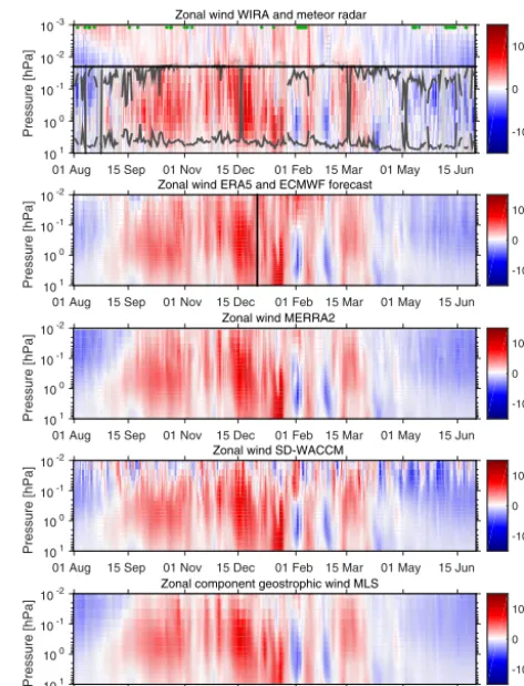
Figure 9.Time series of continuous or near-continuous zonal wind data at Andenes for the time period between 1 August 2016 and 30 June 2017. The green dots in the uppermost panel mark the dates where wind measurements from the RMR lidar are available. The uppermost panel shows wind radiometer data below the horizon-tal black line and meteor radar data above. The dark grey lines in the radiometer data denote the altitude limits within which WIRA data are trustworthy according to the conditions stated in Sect. 2.1. Radiometer data beyond this range are noticeably influenced by a priori assumptions should not be used for comparisons, e.g. with meteor radar observations. At the time of writing ERA5 was only available until 31 December 2016 (black vertical line), and therefore ECMWF forecast data are plotted for 2017.
that all USLM average profiles are based on simultaneous ob-servations and data. As this approach is not possible for the non-overlapping altitude range of the meteor radar, its pro-files are averages over all days. This may lead to slightly dif-ferent temporal sampling between the USLM and the meteor radar data for the tree panels of the summer half-year when WIRA’s uppermost trustworthy altitude is not constantly ad-jacent to the 0.02 hPa line (see Figs. 9 and 10). Moreover, it should be noted that in contrast to the USLM observations meteor radar winds are never convolved with WIRA’s aver-aging kernels according to Eq. (2).
01 Aug 15 Sep 01 Nov 15 Dec 01 Feb 15 Mar 01 May 15 Jun Pressure [hPa] 10-3 10-2 10-1 100 101
Meridional wind WIRA and meteor radar
-100 0 100
01 Aug 15 Sep 01 Nov 15 Dec 01 Feb 15 Mar 01 May 15 Jun
Pressure [hPa]
10-2
10-1
100
101
Meridional wind ERA5 and ECMWF forecast
-100 0 100
01 Aug 15 Sep 01 Nov 15 Dec 01 Feb 15 Mar 01 May 15 Jun
Pressure [hPa]
10-2
10-1
100
101
Meridional wind MERRA2
-100 0 100
01 Aug 15 Sep 01 Nov 15 Dec 01 Feb 15 Mar 01 May 15 Jun
Pressure [hPa]
10-2
10-1
100
101
Meridional wind SD-WACCM
-100 0 100
01 Aug 15 Sep 01 Nov 15 Dec 01 Feb 15 Mar 01 May 15 Jun
Pressure [hPa]
10-2
10-1
100
101
Meridional component geostrophic wind MLS
-100 0 100 W in d s p e e d [m s -1] W in d s p e e d [m s -1] W in d s p e e d [m s -1 ] W in d s p e e d [m s -1] W in d s p e e d [m s -1]
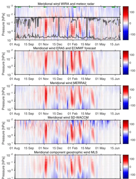
Figure 10.As Fig. 9 but for the meridional wind component.
operational analysis winds between 1 August and 31 Decem-ber 2016 are reprinted in the Fig S5, which confirms that they follow a very similar pattern. Notable differences between ECMWF forecast and ERA5 are, however, found in the zonal and meridional winds above 0.2 hPa for October–November 2016 (Figs. 11 and 12), which according to Fig. S5 are not related to the change of model cycle in the ECMWF fore-casts on 22 November (before this date ECMWF forecast and ERA5 both ran on 41r2) but rather to ERA5 systematically featuring lower absolute zonal and meridional wind speeds at these altitudes.
The fundamental pattern of the time series in Figs. 9 and 10 is the same for all model data and the radiometer observations. Similarly, in cases where the uppermost alti-tude of trustworthy wind radiometer data and the lowermost level of meteor radar observations are adjacent, the handover of the wind profile between these instruments is remarkably smooth without major jumps in the wind profiles. This be-haviour is especially well illustrated for the rapidly changing meridional winds but it can also be discerned for the zonal component.
Despite the good overall agreement of the middle-atmospheric data sources, some differences can be distin-guished.
For instance, the mesospheric westward wind above 0.2 hPa is substantially weaker in the ERA5 reanalysis and the ECMWF forecasts in comparison to WIRA, MERRA2 and the geostrophic wind computations from MLS in Au-gust 2016, which translates to a substantial bias in the upper part of Fig. 11a. SD-WACCM also features comparable wind speeds as the radiometer observations in August, but the strong mesospheric eastward winds around 28 August and 6 September, which could be artefacts, drive the bimonthly av-erage towards zero. Therefrom one might conclude that the advantages of high-altitude input data (MERRA2 and MLS geostrophic wind) or high model tops (SD-WACCM) drive these models closer to the observations than ECMWF.
In the same panel stronger eastward winds of WIRA with respect to all comparison data can be distinguished below 0.4 hPa, where they lie slightly outside the error bands. This is most probably related to the strong eastward winds mea-sured by the radiometer on several consecutive days at the end of August, which are not seen in this strength by any other source of comparison data. The reason for this differ-ence could not be established and unluckily there are no lidar measurements at this time which could provide independent observational evidence.
SD-WACCM features substantially lower zonal wind speeds compared to all data sets and especially to the ob-servations for October–November and December–January above 0.1 hPa. For December–January this tendency seems to be confirmed by the meteor radar wind whereas these are almost equally offset from the high-altitude radiometer and SD-WACCM data for October–November.
Finally, for February–March 2017 ECMWF forecasts, SD-WACCM and radiometer measurements are in close corre-spondence while MLS and the geostrophic winds have off-sets of up to 7 m s−1around 0.1 hPa. Besides these few ex-ceptions the agreement of the zonal wind from the different data sources in Fig. 11 is very good and the comparison data often lie within the error bars of the radiometer.
Regarding the meridional component, winds from all data sources agree with each other and are generally within the observation errors (Fig. 12) for almost all bimonthly av-erage periods. The only notable exceptions occur for SD-WACCM in April–May 2017 with offsets of up to 10 m s−1 and, more pronounced, in February–March 2017, when all comparison data suggest higher winds than observed by the radiometer above 0.2 hPa. Again, the spread between the model data is considerable, with offsets between WIRA and ECMWF extending from 7 m s−1 at 0.1 hPa up to 12 m s−1
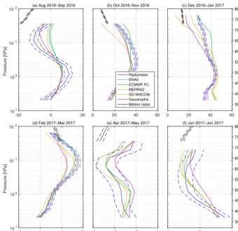
Zonal wind [m s-1]
Approx. altitude [km]
35 40 45 50 55 60 65 70 75 80
-40 -20 0
(f) Jun 2017–Jun 2017
-15 -10 -5 0
(e) Apr 2017–May 2017
-10 0 10 20
Pressure [hPa]
10-2
10-1
100
101
(d) Feb 2017–Mar 2017
Approx. altitude [km]
35 40 45 50 55 60 65 70 75 80
0 20 40 60
(c) Dec 2016–Jan 2017
0 20 40 60
(b) Oct 2016–Nov 2016
Radiometer ERA5 ECMWF FC MERRA2 SD-WACCM Geostrophic Meteor radar
-20 0 20
Pressure [hPa]
10-2
10-1
100
101
(a) Aug 2016–Sep 2016
Figure 11.Bimonthly average profiles of zonal wind at Andenes from reanalyses and models convolved according to Eq. (2) in comparison with observations from the wind radiometer WIRA and its random error (dashed). ERA5 data were only available for the first two panels at the time of writing. At the uppermost altitudes the raw, i.e. unconvolved, meteor radar wind profiles are shown. Due to the temporal variations of the upper altitude limit of the radiometer observations visible in Figs. 9 and 10 the sampling period of the meteor radar average wind can
be rather different from the highest levels of middle-atmospheric data especially for the summer half-year, i.e. in panels(a),(e)and(f).
that the two episodes of strong northward wind at the begin-ning and end of February extend to much higher altitudes in ECMWF than in WIRA data. A similar but reduced tendency is visible for MERRA2. However, the meteor radar observa-tions during these periods seem to confirm the lower velocity meridional winds seen by the radiometer at high altitudes by also showing low adjacent velocities above 0.02 hPa.
In addition to the previously discussed long-term compar-isons, interesting short-term events can be distinguished from the time series. One example shall briefly be discussed here: on 15 and 16 January 2017 a reversal of the zonal wind direc-tion in the mesosphere is clearly visible in the microwave ra-diometer observations in Fig. 9 while the stratospheric winds remain at high eastward velocities. It appears that the tran-sition from the WIRA to the meteor radar profiles is smooth also on these days with the meteor radar winds at the lowest levels also being reverted to westward direction. Moreover, a lidar observation in the night from 14 to 15 January corre-sponded very closely to the radiometer profile (see Fig. S3, second line/second column). Thus, there are good reasons to
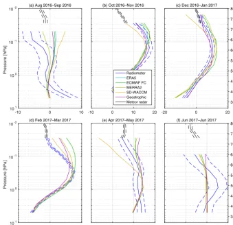
Meridional wind [m s-1]
Approx. altitude [km]
35 40 45 50 55 60 65 70 75 80
-20 -10 0 10
(f) Jun 2017–Jun 2017
-20 -10 0 10
(e) Apr 2017–May 2017
-20 0 20
Pressure [hPa]
10-2
10-1
100
101
(d) Feb 2017–Mar 2017
Approx. altitude [km]
35 40 45 50 55 60 65 70 75 80
-20 0 20
(c) Dec 2016–Jan 2017
-10 0 10 20
(b) Oct 2016–Nov 2016
Radiometer ERA5 ECMWF FC MERRA2 SD-WACCM Geostrophic Meteor radar
-10 0 10
Pressure [hPa]
10-2
10-1
100
101
(a) Aug 2016–Sep 2016
Figure 12.As Fig. 11 but for the meridional wind component.
7 Conclusions
Following the recent developments of the wind measure-ment techniques of Doppler microwave radiometry and lidar iodine absorption spectroscopy, two such instruments have been operated in co-location at Andenes (69.3◦N, 16.0◦E) for an 11-month intercomparison period. After Lübken et al. (2016) had found good correspondence of nighttime lidar winds with eight rocket soundings, the present study can be regarded as the first thorough cross-instrumental validation of the new lidar and radiometry techniques for wind obser-vations in the upper stratosphere and lower mesosphere dur-ing night and day. This part of the study is based on 518 h of coincident observations by the ALOMAR RMR lidar and the microwave radiometer WIRA, with individual record-ings having a minimal duration of 5 h. The intercomparisons have demonstrated the quality of the new measurement tech-niques, which appear to be largely bias-free.
The comparison of the wind observations during sunlit pe-riods prove that the ALOMAR RMR lidar can overcome the additional challenges for daylight operation. Similarly, the nighttime observations confirm that the adjustments to the retrievals presented in Rüfenacht and Kämpfer (2017) allow
wind radiometry to obtain accurate results under both day and night conditions. Particularly the nighttime zonal winds are in very close agreement with all compared data sources, while some differences in the meridional component appear above 0.3 hPa. It should, however, be noted that the over-all nighttime averages are largely dominated by nine con-secutive nights of measurements in February 2017 so that this feature may also be due to a short-term localised effect. During this period the model meridional winds were found to be equally scattered between the radiometer and the li-dar profiles (ECMWF close to lili-dar, SD-WACCM close to WIRA, MERRA2 in between) above 0.3 hPa, indicating no clear preference for either of the observations. Meanwhile the lowermost levels of meteor radar measurements closely correspond to the uppermost radiometer winds.
series correspond very well, as discussed for the 187 h of con-tinuous lidar observations in February 2017.
In conclusion, the observational intercomparisons prove that middle-atmospheric winds from both instruments can be used as single validated standards when operated at dif-ferent sites or as complements when in co-location. In-deed, Doppler radiometry for weather-independent contin-uous monitoring and lidar spectroscopy for high-resolution observations when conditions permit appear to be an ideal combination of measurement infrastructure.
The 11-month time series comparison of quasi-continuous data reveals that the transition from the highest WIRA lev-els to the lowermost radar recordings at around 0.02 hPa is smooth. This statement also applies to the meridional winds in February and March 2017, where the largest discrepan-cies to the models exist. In general the agreement among the different investigated models and reanalyses and with the mi-crowave radiometer observations is very good for both zonal and meridional wind. Nevertheless, examples of pronounced short-term discrepancies between all models and the agree-ing radiometer and lidar measurements have been identified. The most prominent long-term bias has been found in Au-gust 2016 when the westward wind speeds above 0.2 hPa are underestimated by ECMWF’s forecast data and ERA5 re-analyses by up to 10 m s−1 with respect to the radiometer measurements, whereas MERRA2 is in close agreement. To elucidate this difference we aim to target wind radiometer ob-servations to future summers and autumn equinox transitions at high or mid-latitudes, a period which had previously been discounted in view of the rapidly changing winter dynamics.
Appendix A: Validation of mesopause region wind retrievals by WIRA against meteor radar
Rüfenacht and Kämpfer (2017) proposed to exploit the sig-nals recorded by ground-based microwave radiometers oper-ated at ozone emission frequencies to obtain wind informa-tion from the mesopause region. Thanks to the co-locainforma-tion of the wind radiometer WIRA with the Andenes meteor radar the reliability of this approach can be investigated.
It should be noted that microwave radiometry at these al-titudes has some limitations. First of all, observations are only possible at times for which enough emitters (i.e. ozone molecules) are present. This is typically the case during nighttime so that at polar latitudes the retrieval of information about this altitudes is not possible during summer. Moreover, the exact altitude of the signal cannot be determined by the effect of pressure broadening as the linewidth of the emis-sion spectrum at such low pressures is largely dominated by Doppler broadening. This implies that, unlike in the USLM, it is impossible to distinguish signals from different altitudes by their spectral shape. Thus, the attribution of the retrieved wind information to a certain altitude becomes highly de-pendent on the accuracy of the vertical distribution of the mesopause region ozone in the a priori information. In con-trast, meteor radars are specifically designed for observations in the mesopause region and are thus expected to deliver more reliable wind estimates.
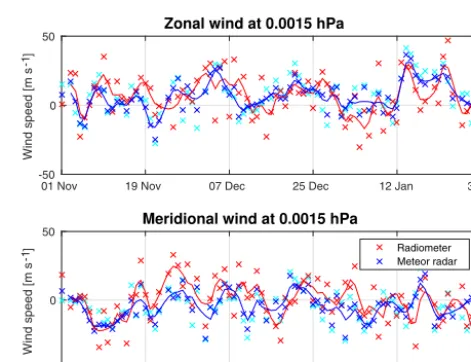
Figure A1 presents the zonal and meridional wind ob-served by WIRA and the Andenes meteor radar during the winter months of 2016/17.
It demonstrates that the mesopause region wind observa-tions by WIRA follow a similar pattern as the meteor radar winds, especially when these are convolved with WIRA’s av-eraging kernels according to Eq. (2). The convolving here not only accounts for the different altitude resolution of the wind radiometer, but, by doing so, also mitigates the effect of possibly inaccurate altitude attributions of the signal as here WIRA’s vertical resolution is basically equivalent to the ver-tical extent of the secondary ozone maximum. From the vali-dation example provided here it may be concluded that in the absence of dedicated co-located instruments for mesopause region wind measurements nighttime wind radiometer data can be used as a source of information for this altitude range.
01 Nov 19 Nov 07 Dec 25 Dec 12 Jan 31 Jan
W
in
d
s
p
e
e
d
[
m
s
-1]
-50 0 50
Zonal wind at 0.0015 hPa
01 Nov 19 Nov 07 Dec 25 Dec 12 Jan 31 Jan
W
in
d
s
p
e
e
d
[
m
s
-1]
-50 0 50
Meridional wind at 0.0015 hPa
Radiometer Meteor radar
Supplement. The supplement related to this article is available online at: https://doi.org/10.5194/amt-11-1971-2018-supplement.
Competing interests. The authors declare that they have no conflict of interest.
Acknowledgements. This work has been funded by the Swiss National Science Foundation grants P2BEP2-165383 and 200020-160048. Moreover the observational part has been supported by the European Union’s Horizon 2020 Research and Innovation programme under grant agreement No. 653980 (ARISE2) and by the German Federal Ministry of Education and Research through the program Role Of The Middle atmosphere In Climate (ROMIC) initiative GW-LCYCLE. We acknowledge ECMWF for the ERA5, the forecasts and the operational analysis data, NASA for the MERRA2 and the Aura MLS data as well as the NCAR CESM working group for providing the SD-WACCM model code.
Edited by: Ad Stoffelen
Reviewed by: two anonymous referees
References
Baldwin, M. P. and Dunkerton, T. J.: Stratospheric harbingers of anomalous weather regimes, Science, 294, 581–584, https://doi.org/10.1126/science.1063315, 2001.
Baron, P., Murtagh, D. P., Urban, J., Sagawa, H., Ochiai, S., Ka-sai, Y., Kikuchi, K., Khosrawi, F., Körnich, H., Mizobuchi, S., Sagi, K., and Yasui, M.: Observation of horizontal winds in the
middle-atmosphere between 30◦S and 55◦N during the
north-ern winter 2009–2010, Atmos. Chem. Phys., 13, 604–6064, https://doi.org/10.5194/acp-13-6049-2013, 2013.
Baron, P., Manago, N., Ozeki, H., Irimajiri, Y., Murtagh, D., Uzawa, Y., Ochiai, S., Shiotani, M., and Suzuki, M.: Measurement of stratospheric and mesospheric winds with a submillimeter wave limb sounder: results from JEM/SMILES and simulation study for SMILES-2, Proc. SPIE, 9639, 96390N-1–96390N-20, https://doi.org/10.1117/12.2194741, 2015.
Baumgarten, G.: Doppler Rayleigh/Mie/Raman lidar for
wind and temperature measurements in the middle atmo-sphere up to 80 km, Atmos. Meas. Tech., 3, 1509–1518, https://doi.org/10.5194/amt-3-1509-2010, 2010.
Baumgarten, G., Fiedler, J., Hildebrand, J., and Lübken, F.-J.: Inertia gravity wave in the stratosphere and mesosphere ob-served by Doppler wind and temperature lidar, Geophys. Res. Lett., 42, 10929–10936, https://doi.org/10.1002/2015GL066991, 2015GL066991, 2015.
Baumgarten, K., Gerding, M., Baumgarten, G., and Lübken, F.-J.: Temporal variability of tidal and gravity waves during a record long 10-day continuous lidar sounding, Atmos. Chem. Phys., 18, 371–384, https://doi.org/10.5194/acp-18-371-2018, 2018. Blanc, E., Ceranna, L., Hauchecorne, A., Charlton-Perez, A.,
Marchetti, E., Evers, L. G., Kvaerna, T., Lastovicka, J., Eliasson, L., Crosby, N. B., Blanc-Benon, P., Le Pichon, A., Brachet, N., Pilger, C., Keckhut, P., Assink, J. D., Smets, P. S. M., Lee, C. F., Kero, J., Sindelarova, T., Kämpfer, N., Rüfenacht, R., Farges,
T., Millet, C., Näsholm, S. P., Gibbons, S. J., Espy, P. J., Hib-bins, R. E., Heinrich, P., Ripepe, M., Khaykin, S., Mze, N., and Chum, J.: Toward an Improved Representation of Middle Atmo-spheric Dynamics Thanks to the ARISE Project, Surv. Geophys., 39, 171–225, https://doi.org/10.1007/s10712-017-9444-0, 2018. Brakebusch, M., Randall, C. E., Kinnison, D. E., Tilmes, S., San-tee, M. L., and Manney, G. L.: Evaluation of Whole Atmosphere Community Climate Model simulations of ozone during Arctic winter 2004–2005, J. Geophys. Res.-Atmos., 118, 2673–2688, https://doi.org/10.1002/jgrd.50226, 2013.
Chanin, M. L., Garnier, A., Hauchecorne, A., and Porteneuve, J.: A Doppler lidar for measuring winds in the
mid-dle atmosphere, Geopys. Res. Lett., 16, 1273–1276,
https://doi.org/10.1029/GL016i011p01273, 1989.
Dragani, R. and McNally, A. P.: Operational assimilation of ozone-sensitive infrared radiances at ECMWF, Q. J. Roy. Meteor. Soc., 139, 2068–2080, https://doi.org/10.1002/qj.2106, 2013.
ECMWF: Changes in ECMWF model, Evolution of the
IFS, available at: http://www.ecmwf.int/en/forecasts/
documentation-and-support/changes-ecmwf-model, last
ac-cess: 12 August 2017a.
ECMWF: Datasets, available at: https://www.ecmwf.int/en/
forecasts/datasets, last access: 12 August 2017b.
Fernandez, S., Rüfenacht, R., Kämpfer, N., Portafaix, T., Posny, F., and Payen, G.: Results from the validation campaign of the ozone radiometer GROMOS-C at the NDACC sta-tion of Réunion island, Atmos. Chem. Phys., 16, 7531–7543, https://doi.org/10.5194/acp-16-7531-2016, 2016.
Fleming, E. L., Chandra, S., Barnett, J., and Corney, M.: Zonal mean temperature, pressure, zonal wind and geopoten-tial height as functions of latitude, Adv. Space Res., 10, 11–59, https://doi.org/10.1016/0273-1177(90)90386-E, 1990.
Forkman, P., Eriksson, P., Winnberg, A., Garcia, R. R., and Kinnison, D.: Longest continuous ground-based measure-ments of mesospheric CO, Geophys. Res. Lett., 30, 1532, https://doi.org/10.1029/2003GL016931, 2003.
Friedman, J. S., Tepley, C. A., Castleberg, P. A., and
Roe, H.: Middle-atmospheric Doppler lidar using an
iodine-vapor edge filter, Opt. Lett., 22, 1648–1650,
https://doi.org/10.1364/OL.22.001648, 1997.
Fritts, D. C., Iimura, H., Lieberman, R., Janches, D., and Singer, W.: A conjugate study of mean winds and planetary waves employing
enhanced meteor radars at Rio Grande, Argentina (53.8◦S) and
Juliusruh, Germany (54.6◦N), J. Geophys. Res.-Atmos., 117,
D05117, https://doi.org/10.1029/2011JD016305, 2012. Froidevaux, L., Livesey, N. J., Read, W. G., Jiang, Y. B., Jimenez,
C., Filipiak, M. J., Schwartz, M. J., Santee, M. L., Pumphrey, H. C., Jiang, J. H., Wu, D. L., Manney, G. L., Drouin, B. J., Waters, J. W., Fetzer, E. J., Bernath, P. F., Boone, C. D., Walker, K. A., Jucks, K. W., Toon, G. C., Margi-tan, J. J., Sen, B., Webster, C. R., Christensen, L. E., Elkins, J. W., Atlas, E., Lueb, R. A., and Hendershot, R.: Early val-idation analyses of atmospheric profiles from EOS MLS on the aura Satellite, IEEE T. Geosci. Remote, 44, 1106–1121, https://doi.org/10.1109/TGRS.2006.864366, 2006.
Gelaro, R., McCarty, W., Suárez, M. J., Todling, R., Molod, A., Takacs, L., Randles, C. A., Darmenov, A., Bosilovich, M. G., Re-ichle, R., Wargan, K., Coy, L., Cullather, R., Draper, C., Akella, S., Buchard, V., Conaty, A., da Silva, A. M., Gu, W., Kim, G.-K., Koster, R., Lucchesi, R., Merkova, D., Nielsen, J. E., Par-tyka, G., Pawson, S., Putman, W., Rienecker, M., Schubert, S. D., Sienkiewicz, M., and Zhao, B.: The Modern-Era Retrospective Analysis for Research and Applications, Version 2 (MERRA-2), J. Climate, 30, 5419–5454, https://doi.org/10.1175/JCLI-D-16-0758.1, 2017.
Hagen, J.: Design and characterisation of a compact 142-GHz-radiometer for middle-atmospheric wind measurements, Mas-ter’s thesis, Faculty of Science, University of Bern, Bern, Switzerland, 2015.
Hersbach, H. and Dee, D.: ERA5 reanalysis is in production, ECMWF Newsletter, p. 7, 2016.
Hildebrand, J., Baumgarten, G., Fiedler, J., Hoppe, U.-P., Kai-fler, B., Lübken, F.-J., and Williams, B. P.: Combined wind measurements by two different lidar instruments in the Arc-tic middle atmosphere, Atmos. Meas. Tech., 5, 2433–2445, https://doi.org/10.5194/amt-5-2433-2012, 2012.
Hildebrand, J., Baumgarten, G., Fiedler, J., and Lübken, F.-J.: Winds and temperatures of the Arctic middle atmosphere dur-ing January measured by Doppler lidar, Atmos. Chem. Phys., 17, 13345–13359, https://doi.org/10.5194/acp-17-13345-2017, 2017.
Hocking, W. K.: Atmospheric Radar: Application and Science of MST Radars in the Earth’s Mesosphere, Stratosphere, Tro-posphere, and Weakly Ionized Regions, Cambridge University Press, Cambridge, 2016.
Hocking, W. K., Fuller, B., and Vandepeer, B.: Realtime de-termination of meteor-related parameters utilizing modern digital technology, J. Atmos. Sol.-Terr. Phy., 69, 155–169, https://doi.org/10.1016/S1364-6826(00)00138-3, 2001a. Iimura, H., Fritts, D. C., Janches, D., Singer, W., and Mitchell, N. J.:
Interhemispheric structure and variability of the 5-day planetary wave from meteor radar wind measurements, Ann. Geophys., 33, 1349–1359, https://doi.org/10.5194/angeo-33-1349-2015, 2015. Jacobi, C.: Meteor radar measurements of mean winds and
tides over Collm (51.3◦N, 13◦E) and comparison with LF
drift measurements 2005–2007, Adv. Radio Sci., 9, 335–341, https://doi.org/10.5194/ars-9-335-2011, 2011.
Kidston, J., Scaife, A. A., Hardiman, S. C., Mitchell, D. M., Butchart, N., Baldwin, M. P., and Gray, L. J.:
Strato-spheric influence on tropospheric jet streams, storm
tracks and surface weather, Nat. Geosci., 8, 433–440, https://doi.org/10.1038/ngeo2424, 2015.
Kishore Kumar, G., Kishore Kumar, K., Baumgarten, G., and Ramkumar, G.: Validation of MERRA reanalysis upper-level winds over low latitudes with independent rocket
sounding data, J. Atmos. Sol.-Terr. Phy., 123, 48–54,
https://doi.org/10.1016/j.jastp.2014.12.001, 2015.
Kopp, M., Gerding, M., Höffner, J., and Lübken, F.-J.: Tidal sig-natures in temperatures derived from daylight lidar soundings
above Kühlungsborn (54◦N, 12◦E), J. Atmos. Sol.-Terr. Phy.,
127, 37–50, https://doi.org/10.1016/j.jastp.2014.09.002, 2015. Kunz, A., Pan, L. L., Konopka, P., Kinnison, D. E., and
Tilmes, S.: Chemical and dynamical discontinuity at
the extratropical tropopause based on START08 and
WACCM analyses, J. Geophys. Res.-Atmos., 116, 1–15, https://doi.org/10.1029/2011JD016686, 2011.
Lamarque, J.-F., Emmons, L. K., Hess, P. G., Kinnison, D. E., Tilmes, S., Vitt, F., Heald, C. L., Holland, E. A., Lauritzen, P. H., Neu, J., Orlando, J. J., Rasch, P. J., and Tyndall, G. K.: CAM-chem: description and evaluation of interactive at-mospheric chemistry in the Community Earth System Model, Geosci. Model Dev., 5, 369–411, https://doi.org/10.5194/gmd-5-369-2012, 2012.
Le Pichon, A., Assink, J. D., Heinrich, P., Blanc, E., Charlton-Perez, A., Lee, C. F., Keckhut, P., Hauchecorne, A., Rüfenacht, R., Kämpfer, N., Drob, D. P., Smets, P. S. M., Evers, L. G., Ceranna, L., Pilger, C., Ross, O., and Claud, C.: Compari-son of co-located independent ground-based middle-atmospheric wind and temperature measurements with Numerical Weather Prediction models, J. Geophys. Res.-Atmos., 120, 8318–8331, https://doi.org/10.1002/2015JD023273, 2015.
Lieberman, R. S., Riggin, D. M., Ortland, D. A., Oberheide, J., and Siskind, D. E.: Global observations and modeling of nonmigrating diurnal tides generated by tide-planetary wave interactions, J. Geophys. Res.-Atmos., 120, 11419–11437, https://doi.org/10.1002/2015JD023739, 2015JD023739, 2015. Livesey, N. J., Read, W. G., Wagner, P. A., Froidevaux, L., Lambert,
A., Manney, G. L., Millan, L., Pumphrey, H. C., Santee, M. L., Schwartz, M. J., Wang, S., Fuller, R. A., Jarnot, R. F., Knosp, B., and Martinez, E.: EOS MLS Version 4.2x Level 2 data quality and description document, Jet Propulsion Laboratory, California Institute of Technology, Pasadena, CA, 2015.
Lobsiger, E.: Ground-based microwave radiometry to deter-mine stratospheric and mesospheric ozone profiles, J. At-mos. Terr. Phys., 49, 493–501, https://doi.org/10.1016/0021-9169(87)90043-2, 1987.
Lübken, F.-J., Baumgarten, G., Hildebrand, J., and Schmidlin, F. J.: Simultaneous and co-located wind measurements in the middle atmosphere by lidar and rocket-borne techniques, Atmos. Meas. Tech., 9, 3911–3919, https://doi.org/10.5194/amt-9-3911-2016, 2016.
Marsh, D. R., Mills, M. J., Kinnison, D. E., Lamarque, J.-F., Calvo, N., and Polvani, L. M.: Climate Change from 1850 to 2005 Simulated in CESM1(WACCM), J. Climate, 26, 7372–7391, https://doi.org/10.1175/JCLI-D-12-00558.1, 2013.
McCormack, J., Hoppel, K., Kuhl, D., de Wit, R., Stober, G., Espy, P., Baker, N., Brown, P., Fritts, D., Jacobi, C., Janches, D., Mitchell, N., Ruston, B., Swadley, S., Viner, K., Whit-comb, T., and Hibbins, R.: Comparison of mesospheric winds from a high-altitude meteorological analysis system and me-teor radar observations during the boreal winters of 2009– 2010 and 2012–2013, J. Atmos. Sol.-Terr. Phy., 154, 132–166, https://doi.org/10.1016/j.jastp.2016.12.007, 2017.
Molod, A., Takacs, L., Suarez, M., and Bacmeister, J.: Development of the GEOS-5 atmospheric general circulation model: evolution from MERRA to MERRA2, Geosci. Model Dev., 8, 1339–1356, https://doi.org/10.5194/gmd-8-1339-2015, 2015.
NASA: Modern-Era Retrospective analysis for Research and Appli-cations, Version 2, Data Access, available at: https://gmao.gsfc. nasa.gov/reanalysis/MERRA-2/data_access, 28 March 2018. NASA: Microwave Limb Sounder, available at: https://mls.jpl.nasa.