OPTIMUM SCHEDULING BASED ON PRICE RESPONSIVE ANALYSIS OF THE RESIDENTIAL MICROGRID

(1)

OPTIMUM SCHEDULING BASED ON

PRICE RESPONSIVE ANALYSIS OF

THE RESIDENTIAL MICROGRID

H. S. PANDYA,

Research Scholar , Electrical Engineering Department,

SardarVallabhbhai National Institute of Technology, Surat 395007, Gujarat, India [email protected]

A.CHOWDHURY

Electrical Engineering Department,

SardarVallabhbhai National Institute of Technology, Surat 395007, Gujarat, INDIA [email protected]

Abstract: This paper presents an approach for optimal scheduling of residential microgrid energy. The proposed mechanism is based on analysis of price responsiveness of residential loads, signature of load peaks are obtained as a response to the different time of use (TOU) tariffs. These signatures are utilized to design optimum tariff plan to obtain effective peak shaving. The price responsive behavior is estimated by particle swarm optimization technique based algorithm that schedules load and renewable generators optimally taking care of climatic conditions and comfort level of the consumers.

Keywords: microgrid; demand response; distributed energy resources; solar photo voltaic; state of charge;

biomass gasifier; time of use; particle swarm optimization

I. Introduction

The residential sector is gaining significance for utility companies in India. Electricity sale to the residential consumers is found while growth of the sector is estimated by 14% over next 10 years [2]. This leads to boost significance of research in residential load pattern analysis, its coincidence factor, time of use and peak-non peak load constraints [1]. It enables utility to estimate price responsiveness of residential load targeting to peak-shaving of overall load profile. The study also found that energy consumption in residential buildings is in the range of 1-3 kWh/m2_{/month, which translates to 12 – 36 annual kWh/ m}2_{and suggests that peak load varies significantly}

between 30-100% based on the prevailing weather conditions [3].

T. Logenthiran, et al.(2012) [4] effectively demonstrated generation scheduling involving micro grid operating in islanding mode. P. Finn, et al.(2013) [5] have proposed peak shaving in residential sector by scheduling renewable energy source viz. wind generator. N. Mehta, et al.(2014) [6] have discussed control of thermostatically controlled loads using strategies based on the timers to control operation so as not to create discomfort but that lead to energy saving. But they did not consider load scheduling, so motivation for consumers to take part in energy exchange with central grid is not addressed. O. Adika st al.(2014) [7] have presented appliance scheduling, by enabling aggregating demand supported by battery storage system so as to avoid peaky system load profile. Manisa Pipattanasomporn et. al.2014)[8], have analyzed residential load by obtaining load profile of various appliances. Hyungna Oh, et. al.(2009) [9] and H.Pandya et al. (2017)[11] have proposed demand-response program tailored to residential customers by analyzing price-sensitive DRP based residential energy management. R.Iyer et. Al [12] have developed smart load control strategy based on energy interface and consumer response.

This work is an effort to study and develop control mechanism for residential loads based on effective tariff design. Scheduling of renewable sources along with the load shifting can make the mechanism more appropriate for the microgrid participants to play active role.

This is an attempt to propose a holistic approach of scheduling price responsive loads as well as renewable sources by implementing Time of Use Tariff (TOU) obtained by detailed price responsive analysis of residential loads targeting towards system peak shaving.

(2)

II. Problem Defination

The problem involves three major layers of functionalities as shown in Fig.1, wherein first and second layers includes process of obtaining TOU by analyzing price responsiveness of different peaks of residential load profile. This TOU is used to prepare final optimum schedule using HPSO.

Fig.1 Basic Algorithm

The data regarding residential load profile is considered from ECO –III-1024[1] reflecting residential load demand pattern of consumers having different income groups and their connected load in Gujarat state in India. A case study using above data was carried out assuming microgrid of 16 homes incorporating consumers of different load profiles in same proportion as in[1]. The consumers, as discussed earlier are considered as prosumers, having rooftop solar PV and biomass gasifier along with a battery storage. The solar PV design and estimation is carried out using PVSys and discussed in the following subsection.

A. Designing roof top solar plant

The system considered here is microgrid connected smart homes wherein one of the renewable sources installed is roof top solar PV system including inverter and battery storage. The system is represented by block diagram as in Fig.2

Fig.2 Block diagram of the solar PV based system

a) Collection of the data:

Site selected for the present case is, place in Ahmedabad city with latitude and longitude of the place that is necessary to obtain the data for the solar radiation of the place. The data regarding radiation, temperature, wind velocity etc. are obtained as per estimated by Meteronorm 7.1. This collected data is used to estimate average hourly, monthly and yearly energy ( kWh ) generated through the assumed system simulated through PVsyst V6.43 for obtaining estimate of electrical energy that can be supplied to the grid and approximate economical analysis of the system

b) Panel orientation and mounting selection:

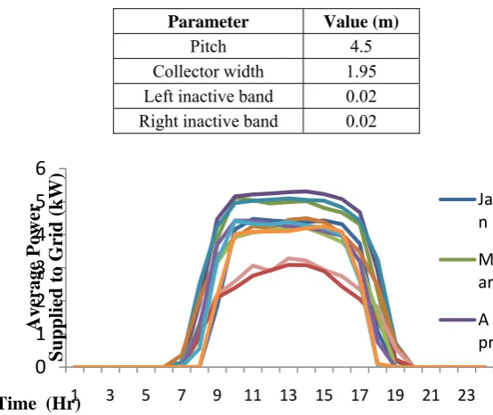
With a view to harvest maximum possible radiation, single axis (N-S) tracking is considered with tilt angle varying at -450_{to 45}0_{. Other parameters are as per Table 1.}

Obtain original demand profile based on the data collection from load estimator/survey

Identify various peaks in load profile and conduct price responsive signature analyze for each peak with change in TOU

Identify optimum TOU and obtain final solution using HPSO based on the same

(3)

Table 1. Heliostats Parameters

C) PV Panel and Inverter selection:

PV Module of Canadian Solar Inc. with 315 Wp is proposed for 8 kW system. Thus 26 modules required to be connected in two parallel string, 13 module in series. While inverter selection is as shown in table 2.

Table 2. PV Module & Inverter Parameters

Fig. 3 Monthly Hourly Average Power Supplied to Grid

Fig.3 depicts monthly hourly power (kW) that can be supplied to grid. It shows that maximum power generated is in April 1:00 pm of 5.31 kW. Average hourly estimated power supplied to grid for April month is used for the case study.

B. Day-Ahead Scheduling Using Hybrid PSO

The scheduling problem that determines two types of decision variables: i) Time flexible or shiftable load demand which needs binary details i.e. to be scheduled or not, at given instant (ON/OFF). And ii) Battery power available at an hour‘t’. This is continuously varying non-binary variable (i.e. continuous variable). Such problem which involves solving continuous as well as binary decision variables (particles), can be solved by Hybrid Particle Swarm Optimization (HPSO) [9]

_bioT

]

.

0

1

2

3

4

5

6

1 3 5 7 9 11 13 15 17 19 21 23

Average Power

Supplied

to Grid (kW)

Time (Hr)

Ja n M ar A pr

No. Of Module 26

Module area 9900 m2

No of Inverters 1

Nominal PV Power 8.19 kwp Maximum PV Power 7.49 kWdc Nominal AC Power 8.0 kWac

Parameter Value (m)

Pitch 4.5

Collector width 1.95

Left inactive band 0.02

(4)

D. Algorithmic steps

The steps involved in preparation of the Swarm, number of variables, swarm sizes, times dimension initialized and defined by the set of randomly generated particles within limits. Repair algorithm fixes the time-constrained variables ON for their ON periods, must-run loads for whole time horizon. Washing machine and flour mill are defined as flexible load without time constraint. Fitness function is constructed for calculating the objective function wherein the profit is calculated.PSO is run to search for the optimal scheduling for the day ahead by scheduling flexible loads, so as to obtain minimum cost to be paid for the consumption, and maximum earning by selling power in peak period, and ultimately obtaining maximum profit. To obtain maximum profit in energy exchange with the utility, the PSO may schedule flexible load demands for minimum time in OFF-peak periods; hence repair algorithm keeps check for the flexible demand should remain ON for the minimum on time expected for the satisfactory operation of particular load.

III. Mathematical Formulation

Above algorithm involved in obtaining optimum schedule for residential load and biomass gasifier so as to obtain maximum profit in the energy exchange day wise considering various constraints is discussed below..

Notations for the formulation are as follows:

t

Hourly time slot for scheduling (hr)

T Total span of scheduling (24 hrs)

h Count of residential consumer

t

G Forecasted solar irradiation at an hour‘t’ (in W/m2)

,

S t

P Hourly power generated by solar PV. (kW)

min

chb

P Minimum permissible state of charge level for battery.

,

chb t

P State of charge of battery at hour‘t’.

min

cr

e b Critical loads energy consumption (in kWh).

max

eb Maximum battery capacity (in kWh).

,

b t

P

Battery power available (in kW), at tth_{hour. (kW)}

,

optl t

P

Total optimized load on the microgrid at an hour ‘t.’(kW)

, ,

l h t

opt

P

Optimally scheduled load demand on the bases of priority of demand at an hour ‘t’ and rate of energy to be drawn from the grid of home ‘h’.(kW)

,

r t



Tariff rate of electrical energy at an houre‘t’. (Rs/kWh)

,

rg t



Tariff rate for electrical energy at an hour‘t’ for drawing energy from grid.(Rs/kWh)

,

rmg t



Tariff rate for electrical energy at an hour‘t’ for supplying energy from micro grid to utility.(Rs/kWh)

chb



Efficiency of battery Charging/discharging operation.

i

x

ith_{particle of the population.}

i

v

Velocity vector.

d

1,2...D dimension of space.

1

,

2

c c

, Two positive acceleration coefficients.

1

R,R₂ Uniformly distributed random numbers in [0, 1].

w

Linearly decreasing function of the iteration index.

max

w

,

w

_min Initial and final weights.

,

biomass t

(5)

, 1

_ _t

u bio _ Scheduled availability of the gasifier.

,

up t



Up time counter. (Hr)

,

dn t



Down time counter. (Hr)

Max up



Maximum up time. (Hr)

Min dn



Minimum down time. (Hr)

bmr



Cost of biomass in Rs/kWh.

Objective function can be defined as:

The objective function targets maximizing profit that is net difference of amount earned from the utility for energy supplied to the grid and amount paid to the utility for energy drawn from the grid.

, , , , , ,

1

((( ) ) ( ( )))

T

S t b t optl t r t biomass t bmr r t t

Maximize P P P



P





     



_{… … …}₍₁₎

Subjected to:

Initial charge: Error! Reference source not found.

,1

chb

P



Initial charge ... ... ...(2)

State of charge dynamics

, , 1 , max

b t chbt chbt

P t P P

eb





  ... … ...(3)

State of charge constraint

min min

,

max 1

cr

ch b ch b t

e b

P P

eb

   ... ... ...(4)

State of battery: charging/discharging:

, ,

,

, ,

1,2,...

Max

b t chb b t b

b t Min

b t chb b t b

P P P

P t T

P P P



     _{ }  

 ... ...(5)

Total load optimized connected to the micro grid at instant‘t’

, optl t

P

= , , 1 1 ( )

l h t

T I opt t h

P

 

 

... ...(6)

Tariff rate of power at time‘t’:



_{r t}_,

, r t



= , , , , , , , , ( ) 1,2,... ( )

rg t s t b t optl t

rmg t s t b t optl t

P P P

t T

P P P



    







… …(7)

Biomass power output: Scheduled output power from biomass gasifier based system to be constrained by the maximum up/down timing as per requirement of the system (discussed in section IV).

… …(8)

… …(9)

Load optimization: total load can be classified and optimized by shifting time-independent load, curtailing less priority loads and controlling thermal (premium loads).

… …(10)

, 1

_

, 1

1,2,...

biomass t biomass t

P

_



P



u bio

_

t



T

, , 1 ,

0

1

Max

up t up

bio t Min

dn t dn

u

















, , , , , , , , , , , ,

l h t fl h t p rl h t th l h t

o p t o p t o p t o p t

m l h t tc l h t

(6)

Where,

P

u u

t

P



P

Fig.4 rep Demand profile ha different. To analy loads for choices. The tariff The sche different , ,

fl i t

opt

P

= opt

other

, , , ,

fl h t

opt

fl h

P



P

,

_ _t

u fl = availa

,

_ 0

1

t

u fl









s

t

= start of pe

f

t

= finish of p

, ,

prl h t

opt

P

= optim

, ,

thl h t

opt

P

= optim

, , , ,

thl h t

opt

thl h

P



ff were floated

eduler has sch load peaks of

imally schedu than the unco

,t



u

_

fl

,t

ability of the f

,

s

f

t t

t t t

 



riod not comf period not com

mally defined a

mally schedule

,t





cycle changes oom, with cha -on load whic

constrained l as per decided

timated daily ogramme (DRP

aks and all pe

ptimal solution profit for eac

d of following

i) Fi

ii) TO

an heduled loads f the original l

uled flexible l omforted perio

1, 2,.

t



flexible load d

f s t t t  

fortable to use mfortable to u

and scheduled

ed thermal loa

... , at given oute ange in therma ch is normally

load which is d during the c

IV.

load profile ba P) offered by aks consisting

n, various sam ch smart home

Fig.4

type: ixed 3 Rs/kW OU with off p nd 9 Rs/kWh.

s responding load profile as

oad: it can be od defined by

..

T

defined by (12

e flexible load use flexible loa

d less priority

ds viz. AC, he

er and inner te al setting for t

critical load i

s non-curtaila contract.

Result and a

ased on the da the given mic g of different t

mple TOU tar e owner with t

4 Original load Pr

Wh, 4 Rs/kWh, peak period 3

change in th s in Fig.5 peak

e scheduled at the user. … ...(11) 2) … …(12) . ad

load, which is

eater which is

... ...(13) emperature di thermal load c in the system.

able load that

analysis

ata input by th crogrid. It also types of load

riff are floated the constraints

rofile

5 Rs/kWh Rs/kWh whil

he tariff rate t ks 1 to 8 are id

t any instant d

s also called c

s defined by (1

fference and t control.

t gets that is

he prosumers d o shows that th their response

d and system s initially set a

e peak load at

that resulted dentified as in

during the tim

curtailable load

13).

thermal insula

operated by

during the reg he original loa e to change in

is allowed to as per their co

t 6 Rs/kWh, 7

in diverse re n Fig.4. me horizon d. ation level consumer istering in ad demand n tariff are

o schedule omfort and

7 Rs/ kWh

(7)

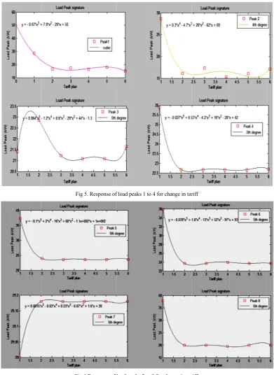
Fig. 5 an signature that insta the types while 5, part of pe

nd 6 shows th es of each pea ant. It is obser s of loads each

6, and 7 are a eak load that i

Fi

hat when PSO ak shows the w

rved that seco h peak consis almost constan is shift-able to

ig 5. Response of

g 6 Response of l

O based sched way load at th ond point in ea sting of. The t

nt. (Peak load o off peak peri

f load peaks 1 to 4

load peaks 5 to 8

duler analyzes hat moment to ach peak sign typical signatu d demand iden iod is called p

4 for change in tar

for change in tar

the price res o be estimated nature takes a ures of peak 1 ntified in Fig. price responsiv

riff

riff.

sponsiveness o d to get vary w big leap whil 1, 2, 3, 4 and 4, changes its veness of peak

of each load p with change in

le next steps d 8 show respo s value by res ks )

(8)

The plots to differe The Load TOU wit to the mi Final shi estimated

s in Fig.7 and ent tariffs men d profile sign th 3 Rs/kWh f

nimum. fted load curv d higher.

Fig. 7

Fig.8 Schedulin

8 show sched ntioned in resp nature plots sh for off peak lo

ve in Fig 9 sh

Scheduling of Bi

ng of Biomass, Ba

duling of biom pective plot. how that out o oad and 7 Rs/k

hows that rem

iomass, Battery e

attery energy and

mass, battery c

of different ta kWh during s

markable peak

nergy and Flexib

Flexible load wit

charging-disch

ariff schemes ystem load pe

shaving can

ble load.

th tariff change 2

harging and fl

applied, it ca eak tariff, all p

be achieved w

2

lexible load in

an be observed peak signature

while profit/d

n response

d that, for es reaches

(9)

Fig.9 Shifted load profile

V. Conclusion

Residential load has a unique characteristics. It consists of less than 25% of load that is automatic and shiftable, others are time dependent.

It is observed that original load profile may be analyzed and by identifying peaks, TOU can be designed. This TOU may be sent as a test signal to the microgrid central controller, which runs the PSO based scheduler simulation constrained by the data collected from the consumers. Itpredicts load response based on TOU. This response is sent to the utility which may finalize TOU for next season or day ahead scheduling by certain trial and analysis.

When TOU is applied, it is observed that flexible loads move to the off peaks reducing overall system peak and whichever load peak consists more non-shiftable loads, consumers are motivated to schedule use of renewable energy sources like PV, biomass and storage. These sources may supply to load during peak periods and also can supply excess energy to the grid.

VI. References

[1] J. U. Amit Garg, Jyothi maheshwari, “Load Research for Residential and Commercial Establishments in Gujarat,” pp. 1–79, 2010. [2] McKinsey, “Powering India :Road to 2017,” McKinsey Co. Mon. J., p. 13, 2008.

[3] M. S. Bhatt, N. Rajkumar, S. Jothibasu, R. Sudirkumar, G. Pandian, and K. R. C. Nair, “Commercial and residential building energy labeling,” vol. 64, no. January, pp. 30–34, 2005.

[4] T. Logenthiran, D. Srinivasan and T. Z. Shun, “Demand Side Management in Smart Grid Using Heuristic Optimization,” vol. 3, no. 3, pp. 1244–1252, 2012.

[5] P. Finn, M. O. Connell, and C. Fitzpatrick, “Demand side management of a domestic dishwasher : Wind energy gains , financial savings and peak-time load reduction,” Appl. Energy, vol. 101, pp. 678–685, 2013.

[6] N. Mehta, N. A. Sinitsyn, S. Backhaus, and B. C. Lesieutre, “Safe control of thermostatically controlled loads with installed timers for demand side management,” ENERGY Convers. Manag., vol. 86, pp. 784–791, 2014.

[7] C. O. Adika and L. Wang, “Electrical Power and Energy Systems Smart charging and appliance scheduling approaches to demand side management,” International Journal of Electric.Power Energy Syst., vol. 57, pp. 232–240, 2014.

[8] M. Pipattanasomporn,et al. “Load Profiles of Selected Major Household and Their Demand Response opportunities,” no. March, 2014. [9] N. Pindoriya, S.Singh, and J.Ostergaard, “Hybrid particle swarm optimization based day-ahead self-scheduling for thermal generator

in competitive electricity market”, in Proc. IFAC Sympo.on Power Plant & Power Syst.control,Tampere,Finland,2009.

[10] X. Guan, Z. Xu, and Q. Jia, “Energy efficient building facilitated by micro grid”, IEEE Trans. Smart Grid, vol.1, no.3, pp. 243-252, Dec. 2010.

[11] H.S.Pandya, A.Chowdhury, “Short Term Scheduling of Rural Residential Electricity Demand by A Smart Micro Grid”,in International Journal of Control Theory and Applications, vol 10, no.6, April 2017.

[12] R.K. Iyer, et al. ““Enabling Smart Distribution System based on Consumer Response and Energy Interface” Second National Conference on Emerging trends in Engineering, Technologyand Management, Jan-2015.

0 5 10 15 20 25

0.5 1 1.5 2 2.5

3x 10

4

X= 23 Y= 20099.2959

Shifted Demand Profile

Time Horizone(Hrs)

P

o

w

e

r(w

)