and scanning radar observations at the Eastern North Atlantic
ARM observatory
Katia Lamer1, Bernat Puigdomènech Treserras2, Zeen Zhu3, Bradley Isom4, Nitin Bharadwaj4, and Pavlos Kollias3,5 1Department of Earth and Atmospheric Science, The City College of New York, New York, USA
2Department of Atmospheric and Oceanic Sciences, McGill University, Montréal, Canada 3School of Marine and Atmospheric Sciences, Stony Brook University, Stony Brook, USA
4Atmospheric Measurement and Data Sciences, Pacific Northwest National Laboratory, Richland, USA 5Department of Environmental and Climate Sciences, Brookhaven National Laboratory, Upton, USA Correspondence:Katia Lamer ([email protected])
Received: 15 April 2019 – Discussion started: 18 April 2019
Revised: 19 July 2019 – Accepted: 6 August 2019 – Published: 11 September 2019
Abstract.Shallow oceanic precipitation variability is docu-mented using three second-generation radar systems located at the Atmospheric Radiation Measurement (ARM) Eastern North Atlantic observatory: ARM zenith radar (KAZR2), the Ka-band scanning ARM cloud radar (KaSACR2) and the X-band scanning ARM precipitation radar (XSAPR2). First, the radar systems and measurement post-processing techniques, including sea-clutter removal and calibration against colo-cated disdrometer and Global Precipitation Mission (GPM) observations are described. Then, we present how a combi-nation of profiling radar and lidar observations can be used to estimate adaptive (in both time and height) parameters that relate radar reflectivity (Z) to precipitation rate (R) in the formZ=αRβ, which we use to estimate precipitation rate over the domain observed by XSAPR2. Furthermore, con-stant altitude plan position indicator (CAPPI) gridded XS-APR2 precipitation rate maps are also constructed.
Hourly precipitation rate statistics estimated from the three radar systems differ because KAZR2 is more sensitive to shallow virga and XSAPR2 suffers from less attenuation than KaSACR2 and as such is best suited for characterizing inter-mittent and mesoscale-organized precipitation. Further anal-ysis reveals that precipitation rate statistics obtained by av-eraging 12 h of KAZR2 observations can be used to approx-imate that of a 40 km radius domain averaged over similar time periods. However, it was determined that KAZR2 is unsuitable for characterizing domain-averaged precipitation rate over shorter periods. But even more fundamentally, these
results suggest that these observations cannot produce an ob-jective domain precipitation estimate and that the simulta-neous use of forward simulators is desirable to guide model evaluation studies.
1 Introduction
Although satellite-based microwave sensors can infer the spatial distribution of liquid water path (Wood and Hart-mann, 2006; Miller and Yuter, 2013) and precipitation rate (Ellis et al., 2009; Adler et al., 2009; Rapp et al., 2013), they have poor horizontal resolution and suffer from surface infer-ence, causing them to under-sample the cloud field variabil-ity and to underreport boundary layer cloud and precipita-tion occurrence (Schumacher and Houze, 2000; Rapp et al., 2013). In contrast, airborne (Stevens et al., 2005; Wood et al., 2011; Moyer and Young, 1994; Vali et al., 1998; Paluch and Lenschow, 1991; Sharon et al., 2006) and ship-based (Yuter et al., 2000; Comstock et al., 2005; Feingold et al., 2010) sensors can resolve the spatial and temporal variabil-ity of the cloud and precipitation field, but field campaigns deploying such sensors are often expensive to conduct and limited in temporal duration (Stevens et al., 2003; Bretherton et al., 2004; Rauber et al., 2007). Island-based observatories, such as the U.S. Department of Energy (DOE) Atmospheric Radiation Measurement (ARM) Eastern North Atlantic ob-servatory (ENA, Mather et al., 2016; Kollias et al., 2016) and the Barbados Cloud Observatory (BCO, Lamer et al., 2015; Stevens et al., 2016), operating profiling and scanning remote sensors can provide long-term statistics of marine light pre-cipitation.
Beyond detecting rain, quantifying the spectrum from drizzle to rain is especially challenging since at small rates droplets are mostly spherical and as such do not generate the typical polarimetric signals required of common precip-itation rate retrievals (e.g., Villarini and Krajewski, 2010; Gorgucci et al., 2000). As an alternative to polarimetric sig-natures, a combination of sensors is typically required to re-trieve precipitation rate (R). Combinations of radar reflectiv-ity (Z) and in situ measurements have led to the develop-ment of Z–R relationships (Wood, 2005; Comstock et al., 2004; VanZanten et al., 2005; Vali et al., 1998); however, these tend not to be universally applicable since they are based on assumptions about the drizzle particle size distri-bution, which may vary with factors such as aerosol load-ing and liquid water path. Moreover, relyload-ing on surface dis-drometer measurements to characterize warm precipitation may be especially unsuitable at the ENA where (i) a large fraction of the precipitation does not reach the surface (Yang et al., 2018), (ii) precipitation reaching the ground typically does so with an intensity below the detection limit of most optical-based disdrometers (∼10−2mm h−1) and (iii) evap-oration is an active process such that water drop size distribu-tion informadistribu-tion retrieved at one height may not be appropri-ate to represent the entire atmospheric column. Alternatively, a method combining radar reflectivity and lidar backscatter measurements has been proposed to retrieve R with fewer assumptions about the drizzle particle size distribution (In-trieri et al., 1993; O’Connor et al., 2005). Because of the current rarity of scanning lidar observations, this technique has only been used to retrieveRin the column and cannot be used to address concerns present in recent studies suggesting
that scanning systems are essential to map domain properties (Oue et al., 2016).
Here we propose exploiting the availability of colocated vertically pointing radar and lidar, as well as scanning radar systems, to characterize marine precipitation rate variability over a domain of 40–60 km around the ENA observatory. The eastern North Atlantic region, with its abundance of marine boundary layer precipitating clouds, is an ideal location for such study (Rémillard and Tselioudis, 2015; Wood, 2012). Observations from the Ka-band ARM zenith radar (KAZR2) and zenith-pointing ceilometer lidar are combined to esti-mate adaptive (both in time and height)Z–R relationships, which we then use to estimate precipitation rate across the domain observed by the X-band scanning ARM precipitation radar (XSAPR2). Domain-averaged and time-averaged pre-cipitation rate estimates obtained from zenith-pointing and scanning observations are compared to document the com-plementarity and applicability of each sensor in documenting precipitation rate from warm boundary layer clouds.
2 Eastern North Atlantic observatory
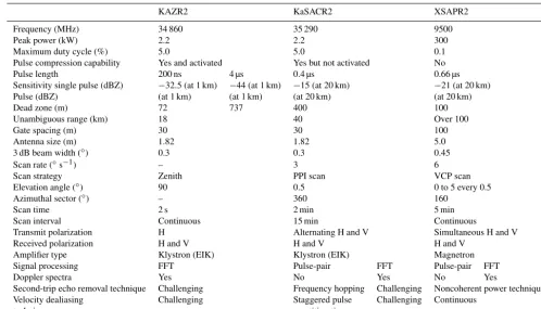
In October 2013, the ARM program established a perma-nent observatory in the eastern North Atlantic on the island of Graciosa (∼60 km2area; 39.1◦N, 28.0◦W). The site, lo-cated in the Azores archipelago, straddles the boundary be-tween the subtropics and the midlatitudes and as such is subject to a wide range of different meteorological condi-tions, including periods of relatively undisturbed trade wind flow, midlatitude cyclonic systems and associated fronts, and periods of extensive low-level cloudiness (Rémillard and Tselioudis, 2015). The observatory hosts an extensive in-strument suite, including three second-generation radar sys-tems: the Ka-band ARM zenith radar (KAZR2), the dual-frequency Ka-band and W-band scanning ARM cloud radar (SACR2) and the X-band scanning ARM precipitation radar (XSAPR2), the specifications of which are listed in Table 1. A short description of the radar systems is provided here with emphasis on changes in configuration from the first to the second generation.
2.1 KAZR2
con-Dead zone (m) 72 737 400 100 Unambiguous range (km) 18 40 Over 100
Gate spacing (m) 30 30 100
Antenna size (m) 1.82 1.82 5.0
3 dB beam width (◦) 0.3 0.3 0.45
Scan rate (◦s−1) – 3 6
Scan strategy Zenith PPI scan VCP scan Elevation angle (◦) 90 0.5 0 to 5 every 0.5
Azimuthal sector (◦) – 360 160
Scan time 2 s 2 min 5 min
Scan interval Continuous 15 min Continuous
Transmit polarization H Alternating H and V Simultaneous H and V Received polarization H and V H and V H and V
Amplifier type Klystron (EIK) Klystron (EIK) Magnetron Signal processing FFT Pulse-pair FFT Pulse-pair FFT
Doppler spectra Yes No Yes No Yes
Second-trip echo removal technique Challenging Frequency hopping Challenging Noncoherent power technique Velocity dealiasing Challenging Staggered pulse Challenging Continuous
technique repetition time
sidering signal integration gain) at ranges from 72 m to 18 km from the radar. KAZR2 has a narrow (0.3◦) 3 dB antenna bandwidth and is nominally operated with a range resolution of 30 m and a temporal resolution of 2 s and is set to record the full radar Doppler spectrum with 256 or 512 fast Fourier transform (FFT) points. KAZR2 transmits a horizontal pulse and receives both horizontal and vertical polarization such that the only polarimetric information it can measure is the linear depolarization ratio.
2.2 SACR2
Ka-band scanning ARM cloud radar (KaSACR2) is a fully polarimetric radar that operates at 35.3 GHz (λ=
8.5 mm) and is an upgraded version of the single polar-ization KaSACR described in Kollias et al. (2014a, b). The KaSACR2 also uses an EIK amplifier with a 2.2 kW peak power and has a 5 % duty cycle and a 3 dB an-tenna beamwidth of 0.3◦. Currently, it is operated with a short pulse, although it could be operated with a longer pulse with pulse compression for increased sensitivity. Ow-ing to its narrow beam width, KaSACR2 must scan rather slowly (3–6◦s−1) to collect observations with a sensitiv-ity of ∼ −15 dBZ at 20 km (not considering signal integra-tion gain). The KaSACR2 conducts a cloud sampling strat-egy that includes different modes (Kollias et al., 2014a, b). Here, because of our interest in mapping precipitation
struc-ture and rate over a large horizontal domain, we use obser-vations collected in plan position indicator (PPI) configura-tion that are only available at 0.5◦ elevation angle over a 160◦ wide azimuth sector. The KaSACR2 conducts a PPI scan every 15 min and takes 2 min to collect each PPI. The KaSACR2 employs frequency hopping and staggered pulse repetition time techniques to mitigate artifacts due to second-trip echoes and velocity aliasing. This, however, comes at the expense of preventing the collection of the full Doppler spec-trum.
2.3 XSAPR2
consid-ering integration gain). The XSAPR2 volume coverage pat-tern (VCP) scan strategy consists of a series of PPI scans every 0.5◦elevation between the angles of 0 and 5◦. Because of considerable beam blockage in the southerly direction, a 160◦ azimuth sector coverage is achieved. The VCP scan (i.e., the entire set of PPI scans) is completed within 5 min and subsequently repeated. Horizontal and vertical polariza-tion are possible for both transmit and receive states, mean-ing XSAPR2 collects a full suite of polarimetric variables while in scanning mode.
3 Radar observations post-processing
Radar observations require considerable post-processing for the removal of non-meteorological targets before they can be scientifically interpreted or used to retrieve geophysi-cal quantities such as precipitation rate. Radar data post-processing is described in Sect. 3.1 and cross-comparison between different systems for calibration is described in Sect. 3.2. Note that the KAZR2 data used for analysis are from “enakazrgeC1.a1” files, KaSACR2 data are from “enakasacrppivhC1.a1” files and the XSAPR2 from the “enaxsaprsecD1.00 files”. All data files were obtained from the ARM archive (https://www.archive.arm.gov/discovery/, last access: 1 September 2019).
3.1 Removal of non-meteorological targets
First, signal processing artifacts (e.g., second-trip echoes) and echoes of non-meteorological origin (e.g., biological echoes, sea clutter and ground clutter) are identified and re-moved.
The KaSACR2 system operates in fully polarimetric mode and uses staggered pulse repetition time and frequency hop-ping to automatically remove second-trip echoes, perform velocity dealiasing and increase the number of independent samples (Pazmany et al., 2013). The XSAPR2 systems oper-ates using a magnetron system that is coherent upon recep-tion (i.e., transmitted pulse phase is random). For the XS-APR2, the removal of second-trip echoes is done using nor-malized coherent power (NCP), which is the coherency of the received pulse with respect to the last transmitted pulse. For atmospheric echoes within the maximum unambiguous range, NCP is high since the radar receiver is phase-locked on the phase of the last transmitted pulse. Outside of the maximum unambiguous range, NCP is low since the radar receiver has already phase-locked on the phase of another transmitted pulse. Here, an NCP threshold of 0.3 is used to identify echoes originating from outside the maximum un-ambiguous range (i.e., second-trip echoes).
Biological targets, such as insects and birds often contam-inate radar observations, especially over land (e.g., Luke et al., 2008). Their occurrence varies with atmospheric condi-tion, time of the year and time of the day (Alku et al., 2015).
KAZR2 observations at the ENA seem minimally impacted by biological echoes. Furthermore, the fact that the bulk of the KaSACR2 and XSAPR2 observations are collected over open ocean and that Graciosa is a small island suggests that biological targets should not be a concern at this particular location.
On the other hand, low-elevation-angle observations are susceptible to sea-clutter contamination. Research on radar sea-clutter characterization and remediation has been ongo-ing for over 20 years (e.g., Horst et al., 1978; Gregers-Hansen and Mital, 2009; Nathanson et al., 1991). Observational and modeling studies suggest that factors such as oceanic wave properties (related to local wind speed and direction), swell and air density streams can affect sea-clutter occurrence. Radar characteristics such as wavelength, wave polarization, beam width and grazing angle are also known to affect sea-clutter characteristics and amounts and our ability to isolate atmospheric returns from sea clutter. Here, observations col-lected over a range of wind conditions during nearly 100 h of clear sky conditions are used to examine how sea-clutter characteristics vary with radar wavelength, beam width and beam elevation angle.
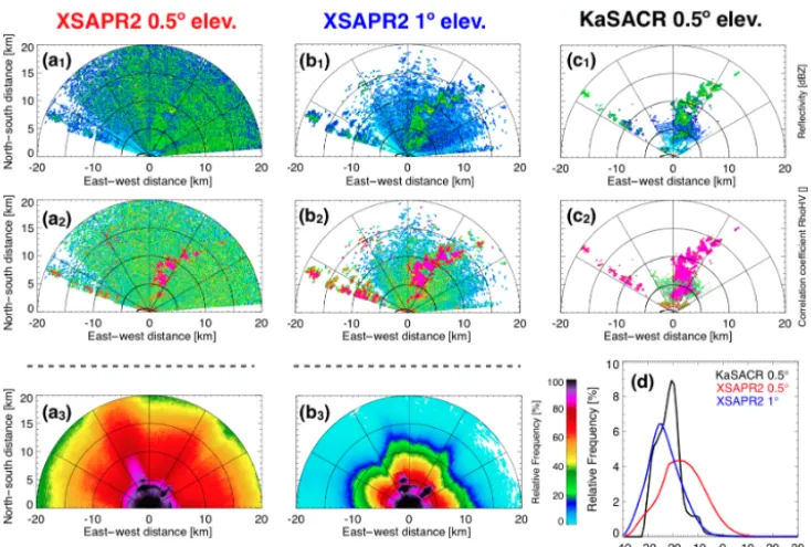
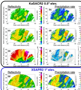
First, the distribution of sea-clutter reflectivities as mea-sured by the XSAPR2 and KaSACR2 at elevation 0.5◦ are compared to document the antenna beam width effect (Fig. 1d). The KaSACR2 (0.3◦ 3 dB antenna beam width) sea-clutter reflectivity distribution is narrower with a peak at
−21 dBZ and a majority of echoes below−15 dBZ (Fig. 1d black line), while the XSAPR2 (0.45◦ 3 dB antenna beam width) sea-clutter reflectivity distribution is wider, peaks at
−18 dBZ and covers a range from−40 to+10 dBZ (Fig. 1d red line). This can be explained by the XSAPR2 wider an-tenna beam width, which results in a larger fraction of the ra-diated energy to hit ocean waves, causing higher ocean clut-ter return power. Similar to beam width, elevation angle af-fects how much sea is in the radar field of view and the spatial extent of observed sea clutter. Figure 1d shows that, at 1.0◦ elevation, XSAPR2 sea-clutter reflectivity peaks at a lower reflectivity of−25 dBZ (blue line) and Fig. 1b3 shows that in this configuration it frequently (> 25 % of the time) de-tects clutter only over a domain of 10 km radius around the site which is much less than it detects when collecting ob-servations at a 0.5◦elevation (significant clutter in a 20 km radius around the site in Fig. 1a3).
Figure 1.For significant echoes, (1) radar reflectivity, (2) correlation coefficient (ρHV) and (3) relative frequency of occurrence of clutter as observed by the(a)XSAPR2 at 0.5◦elevation,(b)XSAPR2 at 1◦elevation and(c)KaSACR at 0.5◦elevation.(d)Clutter characteristics estimated using 93 h of clear sky observations.
dominate both radar reflectivity and correlation coefficient measurements (Fig. 1c1 and c2, respectively). The enhanced KaSACR2 signal-to-clutter ratio is attributed to two effects: (i) its narrow beamwidth, which causes a smaller fraction of the transmitter energy to hit the sea surface, and (ii) its shorter wavelength, which creates a larger distinction be-tween hydrometeor scattering (Rayleigh scattering ∼1/λ4) and sea-clutter (scattering∼1/λ). Using KaSACR2 obser-vations as a guide to locate cloud and precipitation location (Fig. 1c1), it is apparent that it is not possible to distinguish atmospheric signals from sea clutter in XSAPR2 radar reflec-tivity observation collected at 0.5◦(Fig. 1a1).
Several techniques that use both time domain and fre-quency domain filtering methods have been proposed to dis-criminate between sea clutter and meteorological targets in precipitation radar observations (e.g., Torres and Zrnic, 1999; Siggia and Passarelli, 2004; Nguyen et al., 2008; Alku et al., 2015). Ryzhkov et al. (2002) present an echo classification technique based on fuzzy logic and a multiparameter dataset including radar reflectivity, mean Doppler velocity, spectrum width, differential reflectivity, differential phase, linear de-polarization ratio and cross-correlation (ρHV). In the cur-rent study, given the radar’s narrow beam width and short wavelength, an approach solely based on ρHV is used to filter sea clutter. Since cross-correlation between horizontal and vertical cross-polar received powers is largest for spher-ical hydrometeors, we label observations with ρHV larger than a certain threshold as atmospheric returns and the rest
as sea clutter. The analysis of a large sample of ρHV ob-servations during clear and cloudy sky conditions indicates that the use of a threshold of 0.9 for KaSACR2, and an average (over five range gates and five azimuthal measure-ments) threshold of 0.55 for the XSAPR2 can be used to isolate hydrometeor-dominated from clutter-dominated ob-servations. The proposedρHVtechnique successfully isolates atmospheric returns at the same location for both the X band at 1.0◦elevation and the reference Ka band at 0.5◦elevation (Fig. 1b2 and c2, respectively, shown in pink). However, it only identifies a fraction of the atmospheric returns in the X band at 0.5◦elevation observations. There, additional fil-tering, beyond the scope of this study, would be required to suppress the remaining sea clutter and recover the missing atmospheric returns (see Moisseev and Chandrasekar, 2009 and Unal, 2009, who propose advanced techniques). Given this, XSAPR2 cross validation and precipitation rate maps will be estimated using observations collected at 1.0◦ eleva-tion since it offers the best compromise between proximity to the surface and minimum sea-clutter contamination. 3.2 Radar calibration
Figure 2. (a)Ka-band zenith radar (KAZR2) calibration offset to be removed from the KAZR2 radar reflectivity in order to match Parsivel disdrometer radar reflectivity estimates.(b)Ceilometer lidar calibration factor to be multiplied to observed backscatter to match theoretical liquid cloud lidar ratios.(c)Frequency of occurrence of observed backscatter during clear sky conditions, solid black line is interpreted as the mean aerosol backscatter signal, observations smaller than this threshold at each height are eliminated from the drizzle analysis.
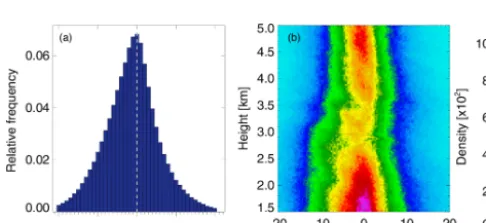
Figure 3.For the period when KAZR2 and KaSACR2 are matched in time and range: (a)difference in radar reflectivity reported by both sensors over the ranges between 1.5 and 5.0 km and the(b) dif-ference in radar reflectivity reported by both sensors as a function of range.
the site. We estimate that, during the period of interest (10 January to 1 April 2018), KAZR2 radar reflectivity mea-surements are off by about +3 dB, which we proceeded to correct for. The detailed time series of KAZR2 calibration offset is presented in Fig. 2a.
Comparison of total (Fig. 3a) and range-resolved (Fig. 3b) histograms of radar reflectivity measured by KAZR2 (pre-calibration) and KaSACR2 at zenith confirm that during the analysis period the KaSACR2 matched KAZR2. For this rea-son, KaSACR2 radar reflectivity measurements were also ad-justed by the calibration constant depicted in Fig. 2a. Note how this comparison between the KAZR2 and KaSACR2 was performed between 1.5 to 5 km to avoid any differences in the reported radar reflectivities due to differences in how they detect ground and sea clutter.
Figure 4.For the conditions that occurred on 4 March 2018 around 09:15 UTC as observed by(a)XSAPR2 radar reflectivity at 1◦ eleva-tion and(c)GPM-DPR Ku-band radar reflectivity at 1 km height. For the entire geometry-matching dataset with 1516 points used for the calibration:(b)scatter, mean (orange) and standard deviation (dashed lines) of the difference between the GPM-DPR Ku band and XSAPR2 radar reflectivity measurements as a function of height and(d)a scatterplot comparing the XSAPR2 and GPM-DPR Ku-band reflectivity measurements above the GPM surface echo height of 1.5 km. Also plotted is the 1-to-1 relationship (dashed line) and the best linear fit to the observations (solid orange line).
with returns smaller than 14 dBZ are not considered dur-ing the comparison procedure (Toyoshima et al., 2015), and only periods when both radar coincidently detect significant precipitation are used to perform calibration. For the analy-sis period, a total of three GPM overpasses with significant precipitation were observed for a total number of 1516 data points for the comparison.
An example of concurrent XSAPR2 and GPM-DPR radar reflectivity observations are shown in Fig. 4a and c, respec-tively. The example shows that both radar detected several shallow precipitation cells with cloud top heights between 3 and 4 km (Fig. 4b). Beyond agreeing in the location of these precipitation echoes, both radar systems (XSAPR2 and GPM-DPR) are found to agree on their reflectivity inten-sity. To confirm their agreement, we estimated the contour of frequency by altitude diagram (CFAD) of the differences in radar reflectivities between the matched XSAPR2 and GPM-DPR for all 1516 available observations (Fig. 4b). Above the height at which GPM-DPR is known to suffer from surface echo contamination (i.e., 1.5 km), the comparison between XSAPR2 reflectivities and GPM-DPR reflectivities shows no noticeable difference (i.e., no bias). A scatter plot between the matched GPM-DPR and XSAPR2 radar reflectivity for heights above 1.5 km confirms the overall lack of bias beyond the expected 1 dB between the two radar at all reflectivities (Fig. 4d, in which the orange line depicts the best fit to the data, the dashed line represents a perfect match between the
datasets and the grey shading indicates the data density). As mentioned above, scatter is expected because of the differ-ences in configuration of both radar systems. The cloud types present in the cases available could further enhance the im-pact of the radar system differences, since the shallow clouds observed during the three overpasses are of similar or even smaller size compared to the GPM-DPR footprint. Small clouds could lead to nonuniform beam filling issues and as such also lead to the GPM-DPR underestimating the reflec-tivity of these cloud systems, which could partially explain the seemingly “high” bias of the XSAPR2 in Fig. 4d. Know-ing that the ARM engineerKnow-ing team had calibrated the XS-APR2 just before the observations used here were collected and because this comparison with the GPM-DPR showed no bias larger than several dB, we conclude that, for the observa-tion period between 10 January to 1 April 2018, the XSAPR2 was reasonably well calibrated and does not require any radar reflectivity adjustments.
4 Radar reflectivity-based precipitation rate retrievals 4.1 KAZR2
Figure 5.Retrieval of popcorn convection precipitation rate on 2 February 2018 using(a)KAZR2 (zenith between 09:30 to 10:30 UTC) and (c)KaSACR2 (1◦elevation PPI at 10:00 UTC). Retrieval of squall line precipitation rate on 2 March 2018 using(b)KAZR2 (zenith between 07:30 to 08:30 UTC) and(d)KaSACR2 (1◦elevation PPI at 08:00 UTC). Also indicated are the location of cloud bases (black dots in panels a–b) and the general wind direction (arrows in panelsc–d). Note that KAZR2 is located at 0 km north–south and east–west.
the width of the water drop size distribution). This radar– lidar technique can be used to estimate precipitation rate at all levels in the subcloud layer when colocated radar and ceilometer observations are available. We apply this tech-nique to the vertically pointing ceilometer lidar and KAZR2 pair operating at the ENA. The O’Connor et al. (2005) technique requires ceilometer backscatter to be calibrated and remapped to the radar spatiotemporal resolution (here 2 s×30 m). Ceilometer backscatter is calibrated following a variation of the O’Connor et al. (2004) technique by scal-ing observed path-integrated backscatter in thick stratocumu-lus to match theoretical cloud lidar ratio values. Satisfactory conditions for ceilometer backscatter calibration are identi-fied as the first (in time) 20 min periods each day with a stan-dard deviation of lidar ratio smaller than 1.5. The observed backscatter during the “satisfactory 20 min period” are input to Hogan (2006)’s multi-scattered model to determine a daily backscatter calibration factor. For days where satisfactory conditions are not observed, a climatological calibration fac-tor of 1.35 is used to calibrate the observed backscatter. For the current analysis period, the ceilometer backscatter cali-bration constant was estimated to vary by around 1.35±0.08 (Fig. 2b). Calibrated ceilometer backscatter is subsequently mapped on the KAZR2 time–height grid using a nearest neighbor approach.
This radar–lidar technique generates time–height maps of precipitation rate from 200 m above ground level to 90 m be-low cloud base height that are filtered for aerosol contamina-tion. We use the clear-sky – according to KAZR2 – calibrated lidar backscatter signals as a reference for aerosol behavior. Lidar-calibrated backscatter values below the mean clear-sky calibrated backscatter value at each height, depicted as the black vertical line in Fig. 2c, are systematically removed from the analysis to leave only drizzle signals. In addition to
aerosol-contaminated returns, unphysical values with a me-dian diameter smaller than 10 µm or equal to or larger than 1000 µm are also removed from our analysis.
Two 1 h examples of cloud location (black dots) and pre-cipitation rate estimated using this technique are shown in Fig. 5a and b. Because of evaporation, the most intense pre-cipitation rates are observed near cloud base height and a significant fraction of the precipitation does not reach the sur-face and falls as virga.
4.2 XSAPR2
As previously mentioned, the estimation of the precipitation rate for the XSAPR2 (i) cannot depend on the use of polari-metric observations because of the absence of polaripolari-metric signature from spherical drizzle drops and (ii) cannot depend on the use of disdrometer-based estimates of the relationship between the radar reflectivity (Z) and the precipitation rate (R) because observations collected at the surface may not be representative of other levels in the subcloud layer, especially at the ENA where evaporation is an active process.
To accommodate changes in drizzle drop size distribution with height, which could be associated, for example, with changes in aerosol loading or evaporation, we propose con-structing adaptive (both with time and height)Z–R relation-ships in the formZ=αRβ from precipitation rates retrieved through the KAZR–ceilometer technique (see Sect. 4.1). Ev-ery 30 min, independently for evEv-ery level in the subcloud layer, retrieved zenith precipitation rates (Rin mm h−1) and calibrated KAZR2 reflectivity (Zin mm6m−3) reported dur-ing a 12 h window around that time are related through the following relationship:
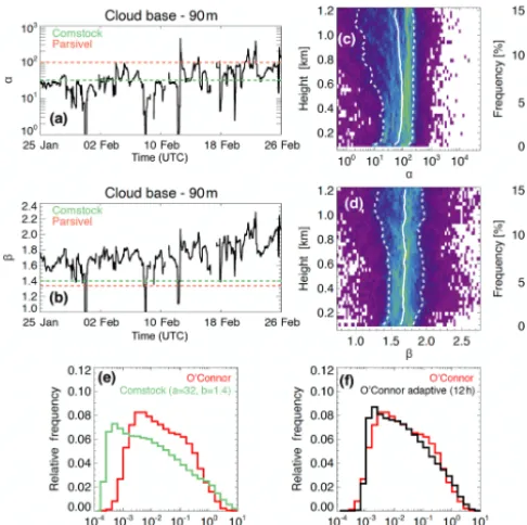
Figure 6.Time series of theα(a)andβ(b)coefficients used to es-timate precipitation rate 90 m below cloud base height for a 30 d pe-riod that overlaps with the second phase of the ACE-ENA field cam-paign. For the same time period, distribution of theα(c)andβ(d) coefficients with height, along with their median (solid line) and 25th and 75th percentile values (dashed line). Precipitation rate dis-tributions retrieved using the O’Connor et al. (2005) technique (red) and estimated using the adaptive coefficients (f, black) or the fixed coefficients proposed by Comstock et al. (2004) (e, green). Com-stock et al. (2004) coefficients and coefficients determined from dis-drometer observations are both presented in panels(a)and(b)using dashed green lines and dashed orange lines, respectively.
The prefactor α and exponent β are estimated using a to-tal least-squares-regression technique only consideringR be-tween 10−3.5and 100.5mm h−1and only if at least 350 pre-cipitation detections are available. When too few observa-tions are available, average (for the period of the current study)αandβare used. A 12 h time window was determined to be the best compromise between data density and the least change in water drop size distribution characteristics.
To evaluate the adaptive Z–R, we apply three different precipitation retrieval techniques to KAZR2 reflectivity ob-servations: we compare precipitation rate statistics retrieved following the O’Connor et al. (2005) technique (ideal tech-nique, red), to those estimated usingZ–Rrelationships con-structed using fixed (approach proposed by Comstock et al., 2004, green) or adaptive (approach proposed here, black) co-efficients (presented in Fig. 6e and f respectively). Figure 6f shows that the proposed adaptiveZ–Rrelationships can re-produce the precipitation rate statistics obtained using the ideal O’Connor et al. (2005) technique. The same cannot be said from using traditional fixed Z–R relationships such as
Figure 7. (a)PPI scan geometry and(b)theoretical sensitivity of the XSAPR2 (blue) and KaSACR2 (black), along with the KaSACR2 “effective” sensitivity, considering it is affected by gas attenuation (green).
that proposed by Comstock et al. (2004), which tends to cre-ate an underestimation of precipitation intensity (Fig. 6e).
Figure 6a and b, respectively, present time series ofαand β near cloud base (i.e., 90 m below cloud base height) for a 30 d period that overlaps with the second phase of the ACE-ENA field campaign. Again, for comparison we illustrate our adaptive coefficients (black), the Comstock et al. (2004) con-stant coefficients (dashed green) and coefficients estimated from surface-based Parsivel laser disdrometer measurements (dashed orange). The gradual increase in both the adaptive αandβ coefficients over time is consistent with reports of observed conditions indicating a transition from shallow pre-cipitation at the end of January to deep frontal prepre-cipitation at the end of February. CFADs ofαandβ (Fig. 6c and d, respectively) show how the adaptiveαadditionally has a ten-dency to increase with distance from cloud base (from top to bottom), which is consistent with the evaporation of small drops that leads to an increase in mean drop size and has been previously reported by Comstock et al. (2004) and discussed in VanZanten et al. (2005).
Figure 8.Example of observations and retrievals of the conditions on 13 February 2018 at 00:10 UTC. Shown for the KaSACR2 when performing 0.5◦elevation PPI are(a)the radar reflectivity field, corrected for gaseous attenuation and neglecting liquid water attenuation, and(b)the corresponding precipitation rate retrieved using adaptiveZ–R relationships;(c)the radar reflectivity field, corrected for both gas and liquid water attenuation and(d)corresponding precipitation rate; and(e)the difference between(a)and(c), showing the range-accumulated radar reflectivity, liquid water attenuation correction, and(f)the corresponding precipitation rate bias. The bottom panels(g) and(h)show simultaneously collected XSAPR2 1.0◦PPI observations for reference.
the ENA observatory, we did not apply any liquid attenuation correction to the XSAPR2 measurements.
4.3 KaSACR2
Before quantitatively estimating precipitation rate from KaSACR radar reflectivity measurements, we also consider how its wavelength responds to the presence of atmospheric gases. The Rosenkranz (1998) propagation model suggests that, for the conditions observed at the ENA, two-way gas attenuation of Ka-band signals can amount to 0.25 dB km−1. Although this may seem small and can be insignificant when collecting observations of boundary layer clouds in profil-ing mode, in scan mode attenuation of Ka-band reflectiv-ity by atmospheric gas can amount to 10 dB at 40 km range
the KaSACR2 “realized” sensitivity does not allow it to de-tect some of the precipitation the more sensitive XSAPR2 can detect. The range-dependent sensitivity of both sensors can be contrasted in Fig. 7b.
5 Radar systems complementarity
As discussed in Sect. 2, the KAZR2, KaSACR2 and XS-APR2 radar sample light precipitation using very different transmission and sampling strategies. In this section we high-light some of the advantages and tradeoffs of using each radar system to characterize different aspects of light precipitation variability.
First, this is done by contrasting the two scanning radar XSAPR2 and KaSACR2. Although the Ka-band SACR2 ex-periences less sea clutter than the X-band SAPR2, it has a coarser temporal resolution; the KaSACR2 only currently performs one PPI scan at 0.5◦every 15 min because it also performs other scan strategies for cloud sampling. In addi-tion, based on their technical specifications (Table 1), the XS-APR2 single pulse radar sensitivity is approximately 10 dB higher than that of the KaSACR2 (Fig. 7b blue and black line, respectively). Finally, the Ka-band SACR2 also suffer from significantly more attenuation from atmospheric gases (Fig. 7b green line) and liquid water, which even if corrected for still decreases its “realized” sensitivity. For all these rea-sons, we conclude that the XSAPR2 is more suitable for char-acterizing light precipitation variability over large domains.
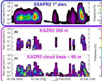
Second, to contrast the XSAPR2 and KAZR2, we com-pare, over the course of 36 h between 00:00 UTC, 2 February, and 12:00 UTC, 3 February, hourly precipitation rate vari-ability in the forms of frequency of occurrence in different precipitation rate bins (pdfs). Figure 9a shows estimates from the scanning XSAPR2 collecting observation in PPI mode covering a domain between 2.5 and 40 km at 1◦ elevation thus transecting heights between∼100 and 750 m (also re-fer to Fig. 7a to visualize the XSAPR2 sampling geometry). Figure 9b and c, respectively, show estimates from the ver-tically pointing KAZR2 200 m above the surface and 90 m below cloud base, which was around 850 m.
From Fig. 9b and c, it is evident that KAZR2, with its high sensitivity, is especially well suited to document light precip-itation and drizzle falling at a rate as low as 10−4mm h−1. KAZR2 observations show a reduction in the number of pre-cipitation events and in prepre-cipitation intensity from cloud
effects. Figure 7a illustrates the height above the surface of a 1◦elevation scan with distance away from the radar; at a distance of 10–20 km the radar beam is already 250 m above the surface while at a distance of 20–30 km this same radar beam is now 500 m from the surface. This nonuniformity of the radar beam height with distance makes scanning cloud radar observations at one elevation angle more adequate to document the character of vertically uniform precipitation. The rapid sampling rate of the KAZR2 also allows it to de-scribe the vertical structure of precipitation variability at a high temporal scale (as short as 2 s).
On the other hand, one drawback of vertically pointing KAZR2 observations is that they are limited to sampling only those precipitation events advected overhead. It is not un-common to temporally average vertically pointing observa-tion to create a proxy for domain-averaged statistics; how-ever, as depicted in Fig. 5, it may be difficult to address the domain representativeness of 1 h of vertically pointing pre-cipitation rate estimates. It can also be challenging to in-terpret the mesoscale organization of the precipitation field using vertically pointing observations alone. Scanning sys-tems such as the XSAPR2 can help fill this gap. Figure 5c and d show XSAPR2 1◦ elevation PPI scans collected at 10:00 and 08:00 UTC, respectively, which corresponds to the center time of the KAZR2 time–height observations pre-sented in Fig. 5a and b. XSAPR2 can observe the structure and scales of popcorn precipitation and squall line precip-itation over a domain of roughly 2500 km2. In its current configuration, the XSAPR2 system can be used to document the horizontal structure and temporal variability of light-to-moderate precipitation on scales of∼5 min. Referring back to Fig. 9a, looking at the hourly precipitation rate pdfs it is evident that by covering a larger domain XSAPR2 is able to observe a larger number of near surface sporadic precipita-tion events such as that observed on 3 February around 00:00 and of isolated deep convective events responsible for more intense precipitation (R>3 mm h−1) such as that observed on 3 February around 08:00.
Figure 9.For a 36 h period (00:00 UTC, 2 February, to 12:00 UTC, 3 February), hourly probability density functions (pdfs) of precipitation rate are presented, estimated from(a)XSARP2 when performing a 1◦elevation PPI scan,(b)KAZR2 200 m from the surface, and(c)KAZR2 90 m below cloud base height.
collected at different elevation angles (i.e., construct con-stant altitude plan position indicator, CAPPI, maps). Here, gridded XSAPR2 CAPPI maps are constructed as follows: we perform the polar to Cartesian transformation for each individual reflectivity measurement using a standard atmo-sphere radio propagation model that considers the height of the beam above the Earth’s surface and the distance between the radar and the projection of the beam along the Earth’s surface (Doviak and Zrnic, 1993). Using these Cartesian co-ordinates each PPI is mapped on a 100 m horizontal grid in which each grid point is populated using a triangulation tech-nique (i.e., the nearest three observations are linearly inter-polated to populate the grid cell). Then, every 100 m in the horizontal, a grid point at constant altitude is populated by (i) a measured value if falling on an elevation where obser-vations were collected or (ii) a weighted average of the grid-ded data from the three closest PPI. The weight being the inverse horizontal distance from the grid location. The afore-mentioned adaptiveZ–Rrelationships are then applied to the Cartesian grid reflectivity observations to produce precipita-tion rate CAPPI. Note that producing an unbiased assessment of precipitation rate over the domain covered by the scanning radar would require the application of a uniform sensitivity threshold over the entire domain. The need for such a thresh-old creates a tradeoff between documenting a large domain and documenting weak precipitation events. As quantified in
Fig. 7b, at a distance of 40 km the XSAPR2 is only capable of detecting precipitation events of an intensity larger than 10−2.8mm h−1and any desire to document weaker precipi-tation rate events would further limit domain size.
7 Domain-averaged precipitation rate – when do temporal and horizontal precipitation variability converge?
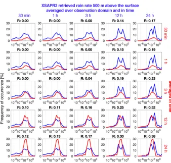
Figure 10.Probability density function of average (over different time windows) precipitation rate as estimated the XSAPR2 and by the KAZR2 (red), both at 500 m above the surface in 100.5mm h−1bins. The XSAPR2 precipitation rates 500 m above the surface being from gridded CAPPI constructed using a collection of PPI scans and limited to the domain between 2.5 and 40 km around the location of the KAZR2. Over each box is the correlation coefficient (R) between the XSAPR2 and the KAZR2 average precipitation rates.
little research has been conducted to determine the validity and limitations of this assumption (see Oue et al., 2016 for a discussion on cloud fraction). In this section we seek to deter-mine how long one needs to observe precipitation advected overhead to gather statistical precipitation information equiv-alent to that of a 40 km radius domain.
Over the 3-month period between 10 January and 1 April 2018, the domain representativeness of KAZR2 pre-cipitation rate estimates is evaluated using XSAPR2 observa-tions collected over a domain of 40 km radius around the site. Although any height could be used, we perform this compar-ison at the specific height of 500 m. While KAZR2 precipita-tion retrievals can be directly extracted at 500 m, those from XSAPR2 must be extracted from gridded CAPPI fields that are constructed following the details provided in Sect. 6 us-ing a collection of PPI scans. To remove any bias caused by variations in minimum performance of both sensors, a mini-mum precipitation rate threshold of 10−2.8mm h−1is applied to both sensors reflecting the detectability of the XSAPR2 over the selected domain. Statistics for both sensors are es-timated using different set averaging time intervals (30 min, 1 h, 3 h, 12 h and 24 h), which allows us to monitor the
tem-poral variability of domain-averaged precipitation rate. For XSAPR2, using a sliding window, we average all 5 min PPI observations collected during the chosen time interval. For KAZR2, we center the time window on the XSAPR2 esti-mates and average all 2 s observations collected during the chosen time interval.
rate pdf from XSAPR2 and 12 h average precipitation rate pdf from KAZR2 are similar in both magnitude and mode location.
Although these results are estimated with few observa-tional cases (3-month period), they clearly suggest that XS-APR2 observations are necessary to characterize short-term (< 1 h) domain-averaged precipitation rate characteristics. They also suggest that longer-term (12 h) domain-averaged precipitation rate characteristics can be estimated by averag-ing either XSAPR2 or KAZR2 observations usaverag-ing time win-dows of similar lengths.
8 Summary and conclusions
The ARM ENA observatory is the first island-based climate research facility equipped with colocated radar and lidar ca-pable of sampling light oceanic precipitation. Here we pre-sented the characteristics and first light observations from three state-of-the-art second-generation radar systems: the Ka-band zenith radar (KAZR2), the Ka-band scanning ARM cloud radar (KaSACR2) and the X-band scanning ARM pre-cipitation radar (XSAPR2).
One of the initial concerns of operating scanning cloud and precipitation radar over the ocean is the impact of sea clutter, especially at low elevation angles. Nearly 100 h of clear sky observations were used to characterize the proper-ties of sea clutter in KaSACR2 and XSAPR2 observations. Analysis of clear and cloudy-sky periods and intercompari-son of the meteorological and non-meteorological echoes of the KaSACR2 made it possible to design a relatively sim-ple filtering technique to isolate precipitation echoes in XS-APR2 observations. In short, a threshold on normalized co-herent power (< 0.3) and on average (5×5 window) cross-correlation (< 0.55) can mitigate second-trip echoes and sea-clutter echoes. Everything considered, we find that XSAPR2 observations collected at 1◦ elevation, albeit suffering from more clutter contamination than KaSACR2, offer the best compromise between clutter contamination and proximity to the surface.
Measurement calibration is also essential to quantita-tive precipitation rate retrieval. We applied the Kollias et al. (2019) technique to calibrate the KAZR2 radar reflec-tivity measurements using Parsivel disdrometer and Cloud-Sat observations. Because they were found to match, the same offset is applied to the KaSACR2 observations. To con-firm the recent calibration performed by the ARM engineer-ing team and to explore alternative calibration methods, the XSAPR2 reflectivity measurements were statistically com-pared to GPM Ku-band radar observations collected around the ENA site. The analysis indicated no noticeable offset; thus, no calibration offset was applied to the XSAPR2. These techniques could be used in the future as a supplement to the ARM radar engineering group efforts to characterize the ENA radar’s reflectivity measurements.
We capitalized on the availability of closely collected (in both time and physical distance) KAZR2, ceilometer lidar and XSAPR2 measurements to estimate precipitation rate. Precipitation rates retrieved using the O’Connor et al. (2005) radar–lidar technique have the advantage of being estimated with fewer assumptions on the drizzle drop size distribution and can accommodate changes in aerosol loading, liquid wa-ter path and evaporation. Unfortunately, due to a lack of scan-ning lidar observations, we cannot apply this technique to scanning radar observations. Instead, we showed how relat-ing the retrieved precipitation rates in the column to radar reflectivity can be used to estimate adaptive (in both time and height) parameters that related observed radar reflectiv-ity (Z) to precipitation rate (R) in the formZ=αRβ. These adaptive parameters can then be applied to retrieve precipi-tation rate over the domain covered by scanning cloud radar systems. We report these adaptive parameters for the period between 10 January and 1 April 2018, which includes the second phase of the ACE-ENA campaign. These adaptive pa-rameters were shown to capture changes in drop size distri-bution with height as well as temporal changes in the cloud field.
Throughout this work, comparison of precipitation rate statistics estimated by all three sensors highlighted the fol-lowing:
1. Because of strong signal attenuation by gases and liq-uid at the Ka band, X-band radar systems are more suited for precipitation mapping, especially over large domains.
2. When the character of precipitation varies rapidly with height, for instance owing to an active evaporation pro-cess, zenith-pointing radar systems are more suited for precipitation characterization.
3. However, zenith-pointing observations collected over periods shorter than 12 h should not be considered rep-resentative of a domain, especially one as large as 2500 km2(i.e.,∼40 km radius half circle).
4. When it comes to capturing the general shape of the pre-cipitation rate distribution, 12 h of zenith-pointing radar observations can be averaged to represent the 12 h vari-ability of a∼40 km radius half circle domain.
5. Shorter-term domain precipitation rate variability can only be captured by scanning precipitation radar sys-tems, in particular those operating at weakly attenuat-ing frequencies and with high sensitivity, such as the XSAPR2.
to observable rain rate through the use of forward simulators, which can use drop size and atmospheric conditions informa-tion to reproduce the attenuainforma-tion affecting radar signals. Sev-eral forward simulators further take into consideration the de-pendency of radar sensitivity with range, which dictates the minimum detectable rain rate at various distances within a domain (e.g., Tatarevic et al., 2015; Lamer et al., 2018).
Data availability. Ground-based data were obtained from the At-mospheric radiation measurement (ARM) user facility, a U.S. De-partment of Energy (DOE) Office of Science user facility managed by the Office of Biological and Environmental Research. Space-borne data were obtained from the National Aeronautics and Space Administration. Column rain rate retrievals were made available by the authors as an ARM PI product.
Author contributions. KL coordinated the project, performed the intercomparisons between the precipitation rates produced by the three radar systems and produced the final manuscript draft. PK su-pervised ZZ and BPT as they, respectively, analyzed the KAZR2 and both the KaSACR2 and XSAPR2 observations. Analysis steps included performing data post-processing, calibration and precip-itation rate retrievals. BPT also produced the CAPPI part of this work. BI and NB provided a wealth of information about the radar system characteristics as well as guidance on radar data calibration. All coauthors read the manuscript draft and contributed comments.
Competing interests. The authors declare that they have no conflict of interest.
Acknowledgements. The authors would like to thank the two anonymous reviewers and Gianfranco Vulpiani for their involve-ment in the review process.
Financial support. Katia Lamer’s contributions were supported by subcontract 300324 of the Pennsylvania State University and the Brookhaven National Laboratory in support of the U.S. Department of Energy (DOE) ARM-Atmospheric Science Research (ASR) Radar Science group. Bernat Puigdomènech Treserras’ contribu-tions were supported through a subcontract with the Brookhaven National Laboratory in support of the ARM-ASR Radar Science group. Zeen Zhu’s contributions were supported by the U.S. DOE ASR ENA Site Science award. Bradley Isom and Nitin Bharadwaj’s
References
Adler, R. F., Wang, J.-J., Gu, G., and Huffman, G. J.: A ten-year tropical rainfall climatology based on a composite of TRMM products, J. Meteorol. Soc. Jpn., 87, 281–293, 2009.
Ahlgrimm, M. and Forbes, R.: Improving the representation of low clouds and drizzle in the ECMWF model based on ARM obser-vations from the Azores, Month. Weather Rev., 142, 668–685, 2014.
Alku, L., Moisseev, D., Aittomäki, T., and Chandrasekar, V.: Iden-tification and suppression of nonmeteorological echoes using spectral polarimetric processing, IEEE T. Geosci. Remote, 53, 3628–3638, 2015.
Bretherton, C. S., Uttal, T., Fairall, C. W., Yuter, S. E., Weller, R. A., Baumgardner, D., Comstock, K., Wood, R., and Raga, G. B.: The EPIC 2001 stratocumulus study, B. Am. Meteorol. Soc., 85, 967–978, 2004.
Comstock, K. K., Wood, R., Yuter, S. E., and Bretherton, C. S.: Reflectivity and rain rate in and below drizzling stratocumulus, Q. J. Roy. Meteor. Soc., 130, 2891–2918, 2004.
Comstock, K. K., Bretherton, C. S., and Yuter, S. E.: Mesoscale variability and drizzle in southeast Pacific stratocumulus, J. At-mos. Sci., 62, 3792–3807, 2005.
Doviak, R. and Zrnic, D.: Doppler Radar and, Academic Press, 562 pp., 1993.
Ellis, T. D., L’Ecuyer, T., Haynes, J. M., and Stephens, G. L.: How often does it rain over the global oceans? The perspective from CloudSat, Geophys. Res. Lett., 36, https://doi.org/10.1029/2008GL036728, 2009.
Feingold, G., Koren, I., Wang, H., Xue, H., and Brewer, W. A.: Precipitation-generated oscillations in open cellular cloud fields, Nature, 466, 849–852, 2010.
Gorgucci, E., Scarchilli, G., and Chandrasekar, V.: Sensitivity of multiparameter radar rainfall algorithms, J. Geophys. Res.-Atmos., 105, 2215–2223, 2000.
Gregers-Hansen, V. and Mital, R.: An empirical sea clutter model for low grazing angles, Radar Conference, 2009 IEEE, 1–5, 2009.
Hogan, R. J.: Fast approximate calculation of multiply scattered li-dar returns, Appl. Optics, 45, 5984–5992, 2006.
Horst, M., Dyer, F., and Tuley, M.: Radar sea clutter model, Anten-nas and Propagation, 6–10, 1978.
Iguchi, T., Seto, S., Meneghini, R., Yoshida, N., Awaka, J., and Kubota, T.: GPM/DPR level-2 algorithm theoretical basis doc-ument, NASA Goddard Space Flight Center, Greenbelt, MD, USA, Tech. Rep, 2010.
Kollias, P., Bharadwaj, N., Widener, K., Jo, I., and Johnson, K.: Scanning ARM cloud radars. Part I: Operational sampling strate-gies, J. Atmos. Ocean. Tech., 31, 569–582, 2014a.
Kollias, P., Jo, I., Borque, P., Tatarevic, A., Lamer, K., Bharadwaj, N., Widener, K., Johnson, K., and Clothiaux, E. E.: Scanning ARM cloud radars. Part II: Data quality control and processing, J. Atmos. Ocean. Tech., 31, 583–598, 2014b.
Kollias, P., Clothiaux, E. E., Ackerman, T. P., Albrecht, B. A., Widener, K. B., Moran, K. P., Luke, E. P., Johnson, K. L., Bharadwaj, N., and Mead, J. B.: Development and applications of ARM millimeter-wavelength cloud radars, Meteor. Mon., 57, 17.11–17.19, 2016.
Kollias, P., Puigdomènech Treserras, B., and Protat, A.: Cal-ibration of the 2007–2017 record of ARM Cloud Radar Observations using CloudSat, Atmos. Meas. Tech. Discuss., https://doi.org/10.5194/amt-2019-34, in review, 2019.
Lamer, K., Kollias, P., and Nuijens, L.: Observations of the vari-ability of shallow trade wind cumulus cloudiness and mass flux, J. Geophys. Res.-Atmos., 120, 6161–6178, 2015.
Lamer, K., Fridlind, A. M., Ackerman, A. S., Kollias, P., Clothiaux, E. E., and Kelley, M.: (GO)2-SIM: a GCM-oriented ground-observation forward-simulator framework for objective evalua-tion of cloud and precipitaevalua-tion phase, Geosci. Model Dev., 11, 4195–4214, https://doi.org/10.5194/gmd-11-4195-2018, 2018. Luke, E. P., Kollias, P., Johnson, K. L., and Clothiaux, E. E.: A
technique for the automatic detection of insect clutter in cloud radar returns, J. Atmos. Ocean. Tech., 25, 1498–1513, 2008. Mather, J., Turner, D., and Ackerman, T.: Scientific maturation of
the ARM Program, Meteor. Mon., 57, 4.1–4.19, 2016.
Matrosov, S. Y.: Attenuation-based estimates of rainfall rates aloft with vertically pointing Ka-band radars, J. Atmos. Ocean. Tech., 22, 43–54, 2005.
Matrosov, S. Y., Kingsmill, D. E., Martner, B. E., and Ralph, F. M.: The utility of X-band polarimetric radar for quantitative es-timates of rainfall parameters, J. Hydrometeorol., 6, 248–262, 2005
Miller, M. A. and Yuter, S. E.: Detection and characterization of heavy drizzle cells within subtropical marine stratocumu-lus using AMSR-E 89-GHz passive microwave measurements, Atmos. Meas. Tech., 6, 1–13, https://doi.org/10.5194/amt-6-1-2013, 2013.
Moisseev, D. N. and Chandrasekar, V.: Polarimetric spectral fil-ter for adaptive clutfil-ter and noise suppression, J. Atmos. Ocean. Tech., 26, 215–228, 2009.
Moyer, K. A. and Young, G. S.: Observations of mesoscale cellu-lar convection from the marine stratocumulus phase of “FIRE”, Bound.-Lay. Meteorol., 71, 109–133, 1994.
Nathanson, F. E., Reilly, J. P., and Cohen, M. N.: Radar de-sign principles-Signal processing and the Environment, NASA STI/Recon Technical Report A, 91, 1991.
Nguyen, C. M., Moisseev, D. N., and Chandrasekar, V.: A para-metric time domain method for spectral moment estimation and clutter mitigation for weather radars, J. Atmos. Ocean. Tech., 25, 83–92, 2008.
O’Connor, E. J., Illingworth, A. J., and Hogan, R. J.: A technique for autocalibration of cloud lidar, J. Atmos. Ocean. Tech., 21, 777–786, 2004.
O’Connor, E. J., Hogan, R. J., and Illingworth, A. J.: Retrieving stratocumulus drizzle parameters using Doppler radar and lidar, J. Appl. Meteorol., 44, 14–27, 2005.
Oue, M., Kollias, P., North, K. W., Tatarevic, A., Endo, S., Vogel-mann, A. M., and Gustafson, W. I.: Estimation of cloud frac-tion profile in shallow convecfrac-tion using a scanning cloud radar, Geophys. Res. Lett., 43, https://doi.org/10.1002/2016GL070776, 2016.
Paluch, I. and Lenschow, D.: Stratiform cloud formation in the ma-rine boundary layer, J. Atmos. Sci., 48, 2141–2158, 1991. Pazmany, A. L., Mead, J. B., Bluestein, H. B., Snyder, J. C., and
Houser, J. B.: A mobile rapid-scanning X-band polarimetric (RaXPol) Doppler radar system, J. Atmos. Ocean. Tech., 30, 1398–1413, 2013.
Rapp, A. D., Lebsock, M., and L’Ecuyer, T.: Low cloud precipi-tation climatology in the southeastern Pacific marine stratocu-mulus region using CloudSat, Environ. Res. Lett., 8, 014027, https://doi.org/10.1088/1748-9326/8/1/014027, 2013.
Rauber, R. M., Stevens, B., Ochs III, H. T., Knight, C., Albrecht, B. A., Blyth, A., Fairall, C., Jensen, J., Lasher-Trapp, S., and Mayol-Bracero, O.: Rain in shallow cumulus over the ocean: The RICO campaign, B. Am. Meteor. Soc., 88, 1912–1928, 2007.
Rémillard, J. and Tselioudis, G.: Cloud regime variability over the Azores and its application to climate model evaluation, J. Cli-mate, 28, 9707–9720, 2015.
Rosenkranz, P. W.: Water vapor microwave continuum absorption: A comparison of measurements and models, Radio Sci., 33, 919– 928, 1998.
Ryzhkov, A., Zhang, P., Doviak, R., and Kessinger, C.: Discrimi-nation between weather and sea clutter using Doppler and dual-polarization weather radars, Proc. 27th General Assembly of the International Union of Radio Science, 3, 2002.
Savic-Jovcic, V. and Stevens, B.: The structure and mesoscale orga-nization of precipitating stratocumulus, J. Atmos. Sci., 65, 1587– 1605, 2008.
Schumacher, C. and Houze Jr., R. A.: Comparison of radar data from the TRMM satellite and Kwajalein oceanic validation site, J. Appl. Meteorol., 39, 2151–2164, 2000.
Sharon, T. M., Albrecht, B. A., Jonsson, H. H., Minnis, P., Khaiyer, M. M., van Reken, T. M., Seinfeld, J., and Flagan, R.: Aerosol and cloud microphysical characteristics of rifts and gradients in maritime stratocumulus clouds, J. Atmos. Sci., 63, 983–997, 2006.
Siggia, A. and Passarelli, R.: Gaussian model adaptive processing (GMAP) for improved ground clutter cancellation and moment calculation, Proc. ERAD, 421–424, 2004.
Stevens, B., Lenschow, D. H., Vali, G., Gerber, H., Bandy, A., Blomquist, B., Brenguier, J.-L., Bretherton, C., Burnet, F., and Campos, T.: Dynamics and chemistry of marine stratocumulus – DYCOMS-II, B. Am. Meteorol. Soc., 84, 579–594, 2003. Stevens, B., Vali, G., Comstock, K. K., Wood, R., Van Zanten, M.
C., Austin, P. H., Bretherton, C. S., and Lenschow, D. H.: Pock-ets of open cells and drizzle in marine stratocumulus, B. Am. Meteorol. Soc., 86, 51–58, 2005.
Unal, C.: Spectral polarimetric radar clutter suppression to enhance atmospheric echoes, J. Atmos. Ocean. Tech., 26, 1781–1797, 2009.
Vali, G., Kelly, R. D., French, J., Haimov, S., Leon, D., McIntosh, R. E., and Pazmany, A.: Finescale structure and microphysics of coastal stratus, J. Atmos. Sci., 55, 3540–3564, 1998.
VanZanten, M., Stevens, B., Vali, G., and Lenschow, D.: Observa-tions of drizzle in nocturnal marine stratocumulus, J. Atmos. Sci., 62, 88–106, 2005.
Villarini, G. and Krajewski, W. F.: Review of the different sources of uncertainty in single polarization radar-based estimates of rain-fall, Surv. Geophys., 31, 107–129, 2010.
Wang, H. and Feingold, G.: Modeling mesoscale cellular structures and drizzle in marine stratocumulus. Part I: Impact of drizzle on the formation and evolution of open cells, J. Atmos. Sci., 66, 3237–3256, 2009.
Warren, R. A., Protat, A., Siems, S. T., Ramsay, H. A., Louf, V., Manton, M. J., and Kane, T. A.: Calibrating ground-based radars against TRMM and GPM, J. Atmos. Ocean. Tech., 35, 323–346, 2018.
Wood, R.: Drizzle in stratiform boundary layer clouds. Part II: Mi-crophysical aspects, J. Atmos. Sci., 62, 3034–3050, 2005. Wood, R.: Stratocumulus clouds, Mon. Weather Rev., 140, 2373–
2423, 2012.
Wood, R. and Hartmann, D. L.: Spatial variability of liquid water path in marine low cloud: The importance of mesoscale cellular convection, J. Climate, 19, 1748–1764, 2006.
nay, C., and Lin, Y.: Clouds, aerosols, and precipitation in the ma-rine boundary layer: An arm mobile facility deployment, B. Am. Meteorol. Soc., 96.3, 419–440, https://doi.org/10.1175/BAMS-D-13-00180.1, 2015.
Yamaguchi, T. and Feingold, G.: On the relationship between open cellular convective cloud patterns and the spatial distri-bution of precipitation, Atmos. Chem. Phys., 15, 1237–1251, https://doi.org/10.5194/acp-15-1237-2015, 2015.
Yang, F., Luke, E. P., Kollias, P., Kostinski, A. B., and Vogelmann, A. M.: Scaling of drizzle virga depth with cloud thickness for ma-rine stratocumulus clouds, Geophys. Res. Lett., 45, 3746–3753, 2018.
Yuter, S. E., Serra, Y. L., and Houze Jr., R. A.: The 1997 Pan Amer-ican climate studies tropical eastern Pacific process study. Part II: Stratocumulus region, B. Am. Meteorol. Soc., 81, 483–490, 2000.
Zhou, X., Heus, T., and Kollias, P.: Influences of drizzle on stratocu-mulus cloudiness and organization, J. Geophys. Res.-Atmos., 122, 6989–7003, 2017.