https://doi.org/10.5194/amt-11-1501-2018 © Author(s) 2018. This work is distributed under the Creative Commons Attribution 4.0 License.
Adaptive selection of diurnal minimum variation: a statistical
strategy to obtain representative atmospheric CO
2
data and its
application to European elevated mountain stations
Ye Yuan1, Ludwig Ries2, Hannes Petermeier3, Martin Steinbacher4, Angel J. Gómez-Peláez5,a,
Markus C. Leuenberger6, Marcus Schumacher7, Thomas Trickl8, Cedric Couret2, Frank Meinhardt9, and Annette Menzel1,10
1Department of Ecology and Ecosystem Management, Technical University of Munich (TUM), Freising, Germany 2German Environment Agency (UBA), Zugspitze, Germany
3Department of Mathematics, Technical University of Munich (TUM), Freising, Germany 4Empa, Laboratory for Air Pollution/Environmental Technology, Dübendorf, Switzerland
5Izaña Atmospheric Research Center, Meteorological State Agency of Spain (AEMET), Santa Cruz de Tenerife, Spain 6Climate and Environmental Physics Division, Physics Institute and Oeschger Centre for Climate Change Research,
University of Bern, Bern, Switzerland
7Meteorological Observatory Hohenpeissenberg, Deutscher Wetterdienst (DWD), Hohenpeissenberg, Germany 8Institute of Meteorology and Climate Research, Atmospheric Environmental Research (IMK-IFU),
Karlsruhe Institute of Technology, Garmisch-Partenkirchen, Germany
9German Environment Agency (UBA), Schauinsland, Germany
10Institute for Advanced Study, Technical University of Munich (TUM), Garching, Germany anow at: Meteorological State Agency of Spain (AEMET), Delegation in Asturias, Oviedo, Spain
Correspondence:Ye Yuan ([email protected])
Received: 29 August 2017 – Discussion started: 12 September 2017
Revised: 1 February 2018 – Accepted: 11 February 2018 – Published: 15 March 2018
Abstract.Critical data selection is essential for determining representative baseline levels of atmospheric trace gases even at remote measurement sites. Different data selection tech-niques have been used around the world, which could po-tentially lead to reduced compatibility when comparing data from different stations. This paper presents a novel statisti-cal data selection method named adaptive diurnal minimum variation selection (ADVS) based on CO2 diurnal patterns
typically occurring at elevated mountain stations. Its capabil-ity and applicabilcapabil-ity were studied on records of atmospheric CO2 observations at six Global Atmosphere Watch
sta-tions in Europe, namely, Zugspitze-Schneefernerhaus (Ger-many), Sonnblick (Austria), Jungfraujoch (Switzerland), Izaña (Spain), Schauinsland (Germany), and Hohenpeis-senberg (Germany). Three other frequently applied statisti-cal data selection methods were included for comparison. Among the studied methods, our ADVS method resulted in a lower fraction of data selected as a baseline with lower
1 Introduction
Continuous in situ measurements of greenhouse gases (GHGs) at remote locations have been established since 1958 (Keeling, 1960). Knowledge of background atmospheric GHG concentrations is key to understanding the global car-bon cycle and its effect on climate, as well as the GHG responses to a changing climate. A critical issue when us-ing data from remote stations remains the identification of time periods that are representative of larger spatial areas and their differentiation from periods influenced by local and regional pollution. If these two regimes are well disag-gregated, the available datasets can represent more reliable information about long-term changes of undisturbed atmo-spheric GHG levels or be used to investigate local and re-gional GHG sources and sinks when specifically analyzing deviations from baseline conditions. In this study, the base-line conditions refer to a selected subset of data from the val-idated dataset, representing well-mixed air masses with min-imized short-term external influences (Elliott, 1989; Calvert, 1990; Balzani Lööv et al., 2008; Chambers et al., 2016).
Measurement results depend on sampling methods, ana-lytical instrumentation, and data processing. Validated data (labeled as VAL in this study to differentiate from the se-lected data) are usually obtained after signal correction, for example due to interferences from other GHGs such as water vapor, calibration accounting for sensitivity changes of the analyzer, and validation based on plausibility checks. Base-line data selection starts with validated data and identifies in subsequent steps a final subset of the validated dataset based on predefined criteria for specific qualities such as represen-tativeness. These data will be referred to as “selected baseline data” or simply as “selected data” in the following.
Data selection methods can be categorized into meteoro-logical, tracer, and statistical selection methods (Ruckstuhl et al., 2012; Fang et al., 2015). Meteorological data selec-tion makes use of the meteorological informaselec-tion at the mea-surement sites, which provides valuable information about the surrounding environment as well as air mass transport (Carnuth and Trickl, 2000; Carnuth et al., 2002). Forrer et al. (2000), Zellweger et al. (2003), and Kaiser et al. (2007) intensively studied the relationship between measured trace gases (such as O3, CO, and NOx)and meteorological pro-cesses at Zugspitze, Jungfraujoch, Sonnblick, and Hohen-peissenberg. For CO2, the most common parameters applied
in the literature are wind speed and wind direction. They can provide information on critical variations at stations with sources and sinks in their vicinity, while these parameters are less suited at stations in largely pristine environments. For example, Lowe et al. (1979) performed a pre-selection on the CO2record at Baring Head (New Zealand) using
pe-riods with southerly winds only (clean marine air). Massen and Beck (2011) found that the CO2versus wind speed plot
can be valuable for baseline CO2estimation without a local
influence of continental measurements. Another widely used
data filtering method is fixed time window selection, by se-lecting data in a certain time interval of the day based on local and mesoscale mechanisms of air mass transport. For selecting well-mixed air at elevated mountain sites, night-time is usually chosen with a special focus on the exclusion of afternoon periods due to the influence of convective up-ward transport (Bacastow et al., 1985). Brooks et al. (2012), for example, limited their mountaintop CO2 results in the
Rocky Mountains (USA) by “time-of-day” from 0 a.m. till 4 a.m. local time (LT) to increase the likelihood of sam-pling the free tropospheric environment at the station. Apart from this, modeling techniques such as backward trajectories are very helpful for analyzing the origins and transport pro-cesses of air masses arriving at the station in detail (Cui et al., 2011). Uglietti et al. (2011) focused on the origins of at-mospheric CO2at Jungfraujoch (Switzerland) by the
FLEX-ible PARTicle dispersion model. Using tracers, data selec-tion can be performed by investigating the correlaselec-tions be-tween the air components of interest. Many tracers have been tested and compared with CO2. Threshold limits of 300 ppb
for CO and 2000 ppb for CH4were defined by Sirignano et
al. (2010) to perform a regional analysis of CO2data at
Lut-jewad (the Netherlands) and Mace Head (Ireland). Similar approaches with black carbon and CH4were performed by
Fang et al. (2015) at Lin’an (China). Moreover, Chambers et al. (2016) applied a data selection technique to identify base-line air masses using atmospheric radon measurements at the stations Cape Grim (Australia), Mauna Loa (Hawaii, USA), and Jungfraujoch (Switzerland).
Unlike most of the methods mentioned above, which re-quire additional data or advanced transport modeling, statis-tical data selection only relies on the time series of interest and typically investigates the variability of signal. It is usu-ally assumed that the most representative CO2data are found
during well-mixed conditions revealing small variations in time (Peterson et al., 1982) and in space (Sepúlveda et al., 2014). For continuous measurements, it is possible to investi-gate within-hour and hour-to-hour variability in the datasets. The within-hour variability is often expressed as the stan-dard deviation of the measured data within 1 h. The hour-to-hour variability compares the differences between hour-to-hourly av-eraged concentrations either during a certain time period, or from one hour to the next. Pales and Keeling (1965) marked ambient data as “variable” when the within-hour variability for the air sample was significantly larger than the within-hour variability for the reference gas. Consequently, they only considered CO2 data to belong to background
condi-tions when the concentracondi-tions were in “steady” condicondi-tions for 6 h or more. Similarly, Peterson et al. (1982) rejected sampled CO2data values for adjacent hours when the
of Baseline Signal”, to estimate the baseline curves general-ized for atmospheric compounds, which is available in the R package IDPmisc (Locher and Ruckstuhl, 2012).
The present study focuses on the comparison of results from previous statistical data selection methods with the new adaptive diurnal minimum variation selection (ADVS) method proposed in this study. The ADVS is seen as a possi-ble alternative to already known data selection methods as discussed above. The results obtained with ADVS for the atmospheric CO2 records from six European mountain
tions are compared with those derived from three other sta-tistical data selection methods. To investigate the potential influences of trend and seasonality, further analyses focus on the decomposition of validated and selected datasets into trend and seasonal components. Finally, differences between ADVS and other data selection methods are assessed by cor-relation analysis.
2 Methods
2.1 CO2measurements at elevated European sites
CO2 measurements from six European mountain stations
(see Fig. 1) within the Global Atmosphere Watch (GAW) network were used. The data were taken from mountain sta-tions due to their remote locasta-tions, being subjected to lim-ited anthropogenic influence and this provided increased rep-resentativeness. Three high alpine measurement sites were included: Zugspitze-Schneefernerhaus (ZSF, DE, 47◦250N, 10◦590E, 2670 m a.s.l.), Jungfraujoch (JFJ, CH, 46◦330N, 7◦590E, 3580 m a.s.l.), and Sonnblick (SNB, AT, 47◦030N, 12◦570E, 3106 m a.s.l.). They are often above the planetary boundary layer (PBL) and thus exposed to free and presum-ably clean lower tropospheric air masses, but periodically influenced by regional emissions from lower altitudes. Ad-ditionally, to test data selection for a less remote environ-ment, CO2measurements were investigated from
Schauins-land (SSL, DE, 47◦550N, 7◦550E, 1205 m a.s.l.) at a much lower elevation, in the mid-range Black Forest. Data selec-tion was also applied to three recently started CO2time series
from different sampling heights above ground on a tall tower at the Hohenpeissenberg observatory (HPB, DE, 47◦630N, 11◦010E, 934 m a.s.l.), located in the northern foothills of the Alps. Henne et al. (2010) presented a method of categoriz-ing site representativeness based on the influence and vari-ability of population and deposition by the surface fluxes. JFJ and SNB were classified as “mostly remote,” while ZSF was considered as “weakly influenced, constant deposition,” and SSL and HPB were considered as “rural” (Henne et al., 2010). Finally, the station Izaña on Tenerife Island (IZO, ES, 28◦190N, 16◦300W, 2373 m a.s.l.) in the North Atlantic was chosen as a reference due to its location above the subtropi-cal temperature inversion layer, which means that the station
is rarely affected by any local or regional CO2sources and
sinks (Gomez-Pelaez et al., 2013).
For this study, unless otherwise indicated, hourly data were used consistently for the purpose of evaluating the data selection method since the method should be easily ap-plicable to data obtained from standard data centers such as the World Data Centre for Greenhouse Gases (WD-CGG) where data are commonly stored with hourly resolu-tion. The validated CO2 hourly averages from all stations
were downloaded from WDCGG (http://ds.data.jma.go.jp/ gmd/wdcgg/). Data with higher time resolution required for some sensitivity analysis in this study were provided directly by the station investigators. All time stamps refer to the be-ginning of the averaging interval. Descriptions of the sam-pling elevation and time period of available data are given in Table 1. Further information on each station can be found in Schmidt et al. (2003) for SSL, Gilge et al. (2010) for HPB and SNB, Gomez-Pelaez et al. (2010) for IZO, Risius et al. (2015) for ZSF, and Schibig et al. (2015) for JFJ. Practi-cal data selections and analyses in this study were performed using the R Statistical Environment (R Core Team, 2017).
2.2 ADVS
ADVS is a tool for automated and systematic analysis of di-urnal CO2 cycles at elevated mountain stations in order to
select consecutive time sequences with minimum variation, which can be regarded as representing well-mixed air con-ditions. Even though such measurement sites are remotely located, the CO2levels are still influenced by local sources
and sinks. For example, at ZSF, these can be characterized by episodic CO2enhancements due to anthropogenic emissions,
detectable especially in winter during the day, whereas in summer the convective upwind transport results in episodes with depleted CO2concentrations due to photosynthetic
up-take of CO2at lower altitudes. Although high altitude
moun-tain stations do not have vegetation in their surroundings, mountain stations at lower altitudes that are still in the vege-tation zone may be influenced by plant respiration, especially at night. As these effects of upward transport photosynthesis and respiration all vary diurnally, the basic strategy that we follow in this study is to identify the most stable time peri-ods of the day, i.e., periperi-ods with minimum variation, which in turn can be used for selecting representative data. How-ever, the duration of this time window during the day varies with the season and from day to day because of variations in the dynamics of transport to the site (e.g., Birmili et al., 2009; Herrmann et al., 2015). In summer, larger variabilities in the CO2signal are observed due to more prevalent
convec-tive boundary-layer air-mass injections influencing the diur-nal pattern, resulting in shorter periods of stable conditions, whereas in winter, significantly longer stable periods occur. No upwind air masses with depleted CO2levels due to
se-Figure 1.Locations of six European elevated mountain stations. Symbols from left to right stand for: IZO – Izaña, Spain; SSL – Schauinsland, Germany; JFJ – Jungfraujoch, Switzerland; HPB – Hohenpeissenberg, Germany; ZSF – Schneefernerhaus-Zugspitze, Germany; SNB – Sonnblick, Austria.
Table 1.Information of measured CO2datasets at six GAW mountain stations.
Station (GAW ID) Sampling elevation (a.s.l.) Time period (yyyy.mm) Data provider
Hohenpeissenberg (HPB) 984/1027/1065 m 2015.09–2016.06 DWD
Schauinsland (SSL) 1210 m 2010.01–2015.12 UBA-De
Izaña (IZO) 2403 m 2010.01–2015.12 AEMET
Zugspitze-Schneefernerhaus (ZSF) 2670 m 2010.01–2015.12 UBA-De
Sonnblick (SNB) 3111 m 2010.01–2015.12 UBA-At
Jungfraujoch (JFJ) 3580 m 2010.01–2015.12 Empa
lect the time window dynamically. ADVS is constructed to select a subset from the measured data, being best represen-tative for baseline conditions with an adaptive selection time window specific for every day.
The algorithm is based on two basic assumptions. First, air masses measured at elevated stations represent well-mixed air, closest to baseline levels, within a certain time window of several hours during the day. For the elevated mountain stations discussed in this paper, this time interval is around midnight. Different diurnal patterns are apparent at each sta-tion, so the selection time window should be adjusted ac-cordingly. Second, it is assumed that real baseline conditions are not subject to local influences and thus represent unper-turbed lower free tropospheric air masses. This indicates that the variability of the measured CO2signal should be minimal
within this selection time window. The methodological steps of ADVS are introduced in detail below in the two sections “starting selection” and “adaptive selection”.
2.2.1 Starting selection
For a given validated hourly dataset, ADVS starts data selec-tion by finding astart time window for all days. The stan-dardized selection procedure for the start time window re-sults from site-specific parameters. This time interval is set as the most stable period from the diurnal variation. The step is referred to asstarting selection. It begins by analyzing the mean diurnal cycle of the data input.
– Step 1: detrending is done by subtracting a 3-day aver-age for each day, including the neighboring two days. It is the shortest possible time window to remove sudden changes in the time series related to the previous and posterior days while preserving the diurnal pattern.
– Step 3: the standard deviations s1j from the overall mean diurnal variation di are calculated on a moving window1j (j=6 h). To be able to place a full set of 24 moving time windows over the overall mean diurnal variation, time windows across midnight (e.g., 6 h from 11 p.m. to 4 a.m. LT) are also included, that is, its first j hours are appended to the end of the 24 h in the over-all mean diurnal variation. The time window with the smallest standard deviation is selected as the start time window.
– Result: the start time window [istart, . . ., iend].
With the focus on elevated mountain stations, starting se-lection is purposely designed with the moving window 1j of 6 h, and the starting houristartto be between 6 p.m. and
5 a.m. LT for this study. For other stations with possibly different diurnal patterns, starting selection can be adjusted accordingly. For instance, at urban stations or stations com-pletely within the continental PBL, the start time window can be chosen based on their best mixing conditions, which often occur in the afternoon with a shorter moving window, when the PBL reaches its maximum depth after “ingesting” free tropospheric air during its growth. Being aware that calculat-ing the start time window from all data could differ from the start time windows calculated by season, the overall gener-ated start time windows have been compared with seasonally generated start time windows for high altitude mountain sta-tions (see Supplement Sect. S1.1). Because these differences were mostly small to moderate and this work aims at a me-thodical comparison under identical conditions, the start time windows are always derived from overall data.
2.2.2 Adaptive selection
The second component,adaptive selection, is designed to de-termine the most suitable time window for each day, based on the data variability. Through this method, the length of the start time window is expanded in both directions in time. Adaptive selection is performed on a daily basis, starting with the first day of the given dataset. The following steps only describe the forward adaptive selection. ADVS also runs thebackward adaptive selectionin an analogous manner but backwards in time.
– Step 1: the mean molar fraction xi, standard devia-tion si, and the proportion of missing values πmissing
are calculated from data in the start time window [istart, . . ., iend].
– Step 2: ifsi≤0.3 ppm (CO2)andπmissing≤0.5, ADVS
continues to advance in time, examine whether the next data pointxf can be included in the selection time win-dow W withf =iend+1. Otherwise, it is considered
that the start time window does not fulfill the assump-tions. In this case, no baseline data is selected for the present day and the algorithm proceeds to the next day.
– Step 3: the absolute difference betweenxf andxi is cal-culated, and the following threshold criterion is applied:
xf−xi
≤κ·si, whereκis the threshold parameter. If this criterion holds,xf is included inWand ADVS con-tinues. Otherwise, ADVS stops for this day with only the start time window, and proceeds to the next day.
– Step 4: mean xW and standard deviation sW for the new selection time windowW are calculated. IfsW≤ 0.3 ppm (CO2), ADVS continues with the next data
pointxf withf =f+1. Otherwise, ADVS stops for this day with the previous selection time window and proceeds to the next day.
– Step 5: the new absolute difference betweenxf andxW is calculated, as well as the new threshold criteria. If condition xf−xW
≤κ·sW holds, xf is included in W and ADVS goes back to Step 4. Otherwise, ADVS stops for this day and proceeds to the next day.
When data selection for all days is finished, ADVS con-tinues with backward adaptive selection. Afterwards, it proceeds to the result.
– Result: this is the final selection time window, which is a combination ofWforwardandWbackwardfor the day in
question.
The following limitations of the forward and backward ex-pansions of the time window should be considered. ADVS always runs for no longer than 24 h including the start time window, i.e.,f ≤24·tr, where tr is the time resolution in data points per hour of the input data. This sometimes results in an overlap of “selected” and “unselected” data for two con-secutive days. We always label the data as “selected” once it has been selected by ADVS. The threshold parameter κ is the controlling factor for the length of the selection time window. Asκincreases, the length of the selection time win-dow increases. A value of 2 was chosen heuristically for this study as a compromise between selecting as many data points as possible and achieving the least data variability. Similar values of sensitivity-controlling parameters in other data se-lection methods can be found (Thoning et al., 1989; Sirig-nano et al., 2010; Uglietti et al., 2011; Satar et al., 2016). In Step 2, values of 0.3 ppm and 0.5 indicate the threshold values forsi andπmissing. We denote them assi,threshold and
πmissing,threshold. Less remote stations at lower altitudes may
require a larger value than 0.3 ppm because of different mix-ing conditions. When performmix-ing ADVS data selection at lower sites such as HPB and SSL, we recommend a higher si,threshold, such as 1.0 ppm. However, throughout this study
we used the described parameter setting (0.3 ppm) for a me-thodical inter-comparison of selection methods at all stations. Potential influences of these parameter sizes (si,threshold and
2.3 Other statistical data selection methods for comparison
We compared ADVS with three statistical data selection methods. The first method named SI is based on “steady in-tervals” (Lowe et al., 1979; Stephens et al., 2013). Steady intervals, which are considered as baseline conditions, are defined by a standard deviation being lower than or equal to 0.3 ppm for six or more consecutive hours. Although this method has some similarity with ADVS, it treats all hours of the day equally without giving preference to hours where the variability is, on average, the smallest.
Second, we adopted a method applied by NOAA ESRL, which originated from Thoning et al. (1989). This se-lection routine has been applied specifically for measure-ments of background CO2 levels at Mauna Loa. This
method (referred to as THO) was applied as described on the website: http://www.esrl.noaa.gov/gmd/ccgg/about/co2_ measurements.html. The first step of THO examines the within-hour variability by selecting hours with hourly stan-dard deviation less than 0.3 ppm. For the hourly data used in this study, the within-hour variability is not applicable so that the first step is skipped. Second, it computes hourly averages and checks the hour-to-hour variability by retaining any two consecutive hourly values where the hour-to-hour difference is less than 0.25 ppm. The last step is based on the diurnal pattern (similar to ADVS), by excluding data from 11 a.m. to 7 p.m. LT due to transported air influenced by photosynthe-sis.
The last method compared is a moving average technique (MA). A moving time window of 30 days and a threshold cri-terion of two standard deviations from the moving averages were applied to discard outliers. Afterwards, new moving av-erages and new threshold criteria were calculated for data exclusion. This step is repeated until no more outliers were found. A more detailed description can be found in Uglietti et al. (2011) and Satar et al. (2016).
2.4 Seasonal-trend decomposition STL
To analyze the results from different data selection methods and compare them with the original validated datasets, we applied the seasonal-trend decomposition technique based on locally weighted regression smoothing (Loess), named STL (Cleveland, 1979; Cleveland et al., 1990). STL has been widely applied to measurements of atmospheric CO2 and
other trace gases (Cleveland et al., 1983; Carslaw, 2005; Brailsford et al., 2012; Hernández-Paniagua et al., 2015; Pickers and Manning, 2015). It decomposes a time series of interest into a trend componentT, a seasonal componentS, and a remainder componentR, which allows detailed sepa-rate analyses of trend and seasonality. Two recursive proce-dures are included in the STL technique: an inner loop where seasonal and trend smoothing based on Loess are performed and updated in each pass, and an outer loop that computes
the robustness weights to reduce the influences of extreme values for the next run of the inner loop (Cleveland et al., 1990).
For this study, we used the implemented function stlin R (R Core Team, 2017). Owing to functional limitation of
stl, full time coverage of monthly data is needed in order to reduce the risk of large time gaps or unequal spacing (Pick-ers and Manning, 2015). All data were first aggregated to monthly averages. Then, missing data were substituted by linear interpolation, using R functionna.approx(Zeileis and Grothendieck, 2005). For the application of STL, two param-eters need to be specified, which are the seasonal smooth-ing parametern(s) (s-window in functionstl) and the trend smoothing parametern(t) (t-window in functionstl). Asn(s) and n(t) increase, the seasonal and trend components get smoother (Cleveland et al., 1990). For optimal compatibility in this study, the same parameters were chosen for all stations asn(s)=7 and n(t)=23, based on the recommendation of Cleveland et al. (1990). Another parameter combination of n(s)=5 andn(t)=25 was also tested according to Pickers and Manning (2015), but with no significant differences in results.
3 Results and discussion
3.1 Start time window
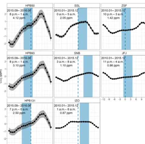
ADVS was applied to the validated hourly averages from all six stations with the parameter settings as described above. The detrended mean diurnal cycles were obtained together with the start time window for each station by starting se-lection (see Fig. 2, for conventional mean diurnal plots see Supplement Sect. S2). The observed differences in the start time windows, as well as in the widths of the confidence in-tervals (gray shades), reflect the characteristics of differently situated measurement sites and different sampling levels. The first subplot column (HPB50, HPB93, and HPB131), repre-senting the three sampling heights at HPB, shows similar de-trended diurnal patterns with similar start time windows. The slightly different start time window at HPB131 potentially indicates different dynamics of the atmospheric transport at higher elevation. The decreasing amplitude with increasing sampling height indicates that the higher the sampling inlet is above the ground, the less it is affected by the local sur-face fluxes. The three start time windows suggest that the most stable period at HPB occurs during the last few hours of a day, including midnight. However, in contrast to all other stations covering at least a full year, HPB data are only from September of 2015 to June of 2016. The results may not be fully comparable, but instead it shows that the data selection method is also applicable to data with time periods shorter than one year.
Figure 2.Detrended mean diurnal cycles of validated CO2datasets (black) with 95 % confidence intervals (gray) from six GAW sta-tions (hours in LT). Measurements at HPB are differentiated by the sampling heights (e.g., HPB50 for 50 m a.g.l.). The covered time periods (top text), resulting start time windows (middle text, also in light blue shades), and mean diurnal amplitudes (bottom text) are shown in each subplot.
on or later in the morning. The start time window for SSL encompasses its diurnal maximum, indicating that data vari-ability is considerably smaller in the early morning than in the afternoon because of its vicinity to the Black Forest re-gion, which has strong influence due to local photosynthetic activity (Schmidt et al., 2003). A similar diurnal pattern can be found at SNB. The influence of CO2 sources is not as
prominent as the effect of distant CO2sinks, since it is
sit-uated at the isolated summit peak of Hoher Sonnblick sur-rounded only by mountains and glaciers, with a negligibly small number of tourists, thus anthropogenic activities are minimal. IZO is a special case, since it is located on a re-mote mountain plateau on the Island of Tenerife above the strong subtropical temperature inversion layer. Even though the start time window is limited to 6 h, IZO presents an ideal mean diurnal cycle for data selection from a potentially much longer time window.
In the right column of the figure, both ZSF and JFJ find their start time windows around midnight (including hours after midnight). ZSF shows higher diurnal CO2 amplitude
than JFJ, but the two sites show similar diurnal patterns. For the choice of the start time window from the mean di-urnal variation, relatively close or even local anthropogenic sources may influence the CO2at these two stations, possibly
due to touristic influences.
Figure 3.Time series plots of validated CO2datasets (gray), and
selected datasets by ADVS (black) at six GAW stations.
3.2 Percentage of selected data
Starting from the initial start time windows, ADVS selected the baseline data for all stations (see Fig. 3). In addition, we calculated the percentages of the complete datasets se-lected by ADVS as baseline data, which are listed in the first column of Table 2. The higher the percentage the more well-mixed air is measured at the station, which is assumed to be a representation of lower free tropospheric conditions. This holds especially for IZO, where a larger percentage of 36.2 % was selected as baseline data. The sites with interme-diate percentages are JFJ (22.1 %), SNB (19.3 %), and ZSF (14.8 %). For the three sampling heights at HPB, only 3.2 % (50 m), 4.8 % (93 m), and 6.2 % (131 m) of the data were selected by ADVS. Finally, a similarly low percentage was found for SSL (4.0 %), probably due to its higher data vari-ability.
ab-Table 2.Percentage of selected data in all data by different data selection methods. The bottom shows the linear regression coeffi-cients of station (HPB is represented by HPB50; IZO is excluded) altitudes and the percentages of selected data at the significance level of 0.05 (∗∗∗).
Station ID ADVS SI THO MA
HPB50 3.2 13.9 21.7 79.8
HPB93 4.8 18.5 25.0 79.4
HPB131 6.2 21.3 27.3 79.8
SSL 4.0 17.9 25.4 83.2
IZO 36.2 82.2 56.0 60.5
ZSF 14.8 47.1 40.8 79.0
SNB 19.3 58.7 44.2 76.9
JFJ 22.1 62.1 46.3 77.6
Linear regression 0.996∗∗∗ 0.992∗∗∗ 0.985∗∗∗ 0.645 coefficient (γ2)
solute altitudes and the percentages of selected data for con-tinental stations. IZO is on a remote island and therefore not comparable. This approach reveals a significant positive lin-ear trend (see coefficient in Table 2). The related figure of linear regression can be found in Supplement Sect. S3.1.
To examine the characteristic growth of the percentages of selected data by ADVS during the selection process, we ad-ditionally calculated percentages after completing both the starting selection and adaptive selection steps mentioned in Sect. 2.2 (see Supplement Sect. S3.2). All results of percent-ages show an order of stations similar to that above, and the percentages increase steadily step by step for all stations. The percentages of selected data by ADVS were then compared with those of the mentioned statistical data selection meth-ods SI, THO, and MA (see Table 2, with the corresponding figure shown in Supplement Sect. S3.3).
Since the percentages of selected data indicate not only the amount of data declared as representative but also show the characteristics of the selection methods, this criterion is used for further assessment. All other methods except for MA result in higher percentages for higher altitude stations (IZO, ZSF, SNB, and JFJ) than for those of lower altitudes (HPB and SSL). ADVS always performs the strictest filter-ing in all cases. Based on the stepwise study (see Supplement Sect. S3.2), these low percentages are primarily due to the restrictive definition of the start time window requiring data with a standard deviation of less than 0.3 ppm. With adap-tive selection, the percentages of selected data increase but remain lower than those of the other methods. SI and THO, in comparison, show differences between stations at high and low elevations. Compared with SI, THO is higher at stations at lower elevations, but lower at high ones. A major limita-tion of SI seems to be the requirement for consecutive hours, in our case of 6 h with 0.3 ppm standard deviation threshold, which might be too restrictive for stations at lower elevations. However, this criterion results in a fairly large percentage for
stations at high elevations. At ZSF, SNB, and JFJ, it results in the second largest, and even the largest in the case of IZO. The highest percentages of selected data (approximately 80 %) were obtained with MA at most stations except for IZO. However, IZO obtains the largest percentages from all other selection methods. This is probably caused by the very low variability of CO2at IZO, resulting in overly strict
moving-average thresholds for the MA method. Thus, we conclude that MA does not work properly in the case of very well-mixed air (IZO). At all other stations, it is possible that MA declares too much data as representative. Therefore, MA was excluded from further analyses.
3.3 STL components
STL was applied to the validated datasets before and after baseline selection with SI, THO, and ADVS, except for HPB due to its limited length of time (less than one year). Depend-ing on data availability, STL was performed on CO2 data
from 2012 to 2015 at SNB, while data inputs at SSL, IZO, ZSF, and JFJ cover the whole period from 2010 to 2015. Fig-ure 4 gives an overview of the decomposition by STL. The following sections discuss the resulting components obtained by STL, namely the trend component, the seasonal compo-nent, and the remainder component.
3.3.1 Trend component
From the trend components, the mean annual growth rates were estimated by linear regression (see Table 3). Based on the 95 % confidence intervals for the slope, positive trends i.e., increasing CO2 concentrations are observed. Owing to
the overlap of the confidence intervals, differences in the mean annual growth rates among VAL and selected datasets at the same station are all in good agreement. This indicates that the trend component is not significantly influenced by the statistical data selection method, which agrees well with the finding of Parrish et al. (2012) from a study of baseline ozone concentrations that there were no significant differ-ences of the long-term changes between the baseline and un-filtered datasets. Moreover, the following fact is observed for all sites except for SSL. Compared to unselected data (VAL), the mean annual growth rates based on selected datasets are systematically higher approaching the growth rates at IZO. IZO can be considered as better representing the lower free tropospheric conditions and agrees well with the mean an-nual global CO2 growth rates (2.31 ppm) during the same
Figure 4.STL decomposition results from VAL (black), SI-selected (brown), THO-selected (yellow), and ADVS-selected (green) datasets at five GAW stations.
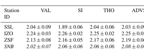
Table 3.Mean annual growth rates (ppm yr−1)with 95 % confi-dence intervals from linear regression, applied on the trend com-ponents by STL over 2010 to 2015, except for SNB. Data at SNB were decomposed over 2012 to 2015 due to missing data from 2010 to 2011 and thus shown in italic font.
Station VAL SI THO ADVS
ID
SSL 2.04±0.09 1.89±0.06 2.04±0.06 2.03±0.09 IZO 2.24±0.03 2.26±0.02 2.25±0.02 2.25±0.02 ZSF 2.13±0.08 2.16±0.05 2.17±0.06 2.19±0.06
SNB 2.02±0.07 2.06±0.06 2.06±0.06 2.08±0.04
JFJ 2.13±0.03 2.15±0.02 2.14±0.02 2.14±0.02
3.3.2 Seasonal component
The resulting seasonal components show systematic differ-ences between VAL and selected datasets. The mean monthly variations were calculated on a monthly scale over the en-tire period from the analyzed data. Figure 5a and b present the results at stations ZSF and IZO. At most stations (except for IZO), the seasonal amplitudes have been substantially re-duced compared to VAL (see also Fig. 4). At ZSF, the aver-aged peak-to-peak seasonal amplitude, defined as mean sea-sonal maximum minus seasea-sonal minimum, drops the most by 18.9 % from VAL with the ADVS selected dataset. An expla-nation of this reduction is CO2 signal exclusion from local
sources and sinks by data selection. When taking a closer look at the monthly averages, lower CO2 values are found
in the selected datasets in the winter months from October to April, indicating that the CO2 concentrations estimated
by VAL are above the background levels because of more dominant anthropogenic activities and no active vegetation.
Higher values in the summer months from May to September explain underestimation of VAL due to intensified upward transport of photosynthetic signatures resulting from vege-tation. Similar patterns can be found at stations SSL, SNB, and JFJ (see Supplement Sect. S4). IZO always shows the smallest seasonal amplitude and there is almost no difference between VAL and selected datasets. Based on this consider-ation, it is very likely that the lower free troposphere will react with a delay to CO2concentration changes of effective
sources and sinks on the ground, acting like an atmospheric memory.
Figure 5.Mean monthly variation of the seasonal component decomposed by STL at(a)ZSFand(b)IZOover the whole period. For a better visualization of the results of selection methods, dots have been separated horizontally and equidistantly. The 95 % confidence intervals are shown as error bars.
found it representative for the free tropospheric air by ana-lyzing the annual and diurnal cycles. From spring onwards, the PBL rises with increasing temperatures. The intense ver-tical atmospheric exchange during summer months results in a daily air mass transport from the boundary layer to reach ZSF due to thermal convection (Reiter et al., 1986; Birmili et al., 2009). Thus there are optimal transport and mixing con-ditions. Therefore after data selection, the timing of seasonal peaks corresponds better among the stations.
3.3.3 Remainder component
The remainder component resembles random noise from lo-cal influences in its structure, being different from site to site and statistically uncorrelated with the general signal of CO2
concentrations in the lower free troposphere (Thoning et al., 1989). The standard deviation of the remainder component is taken here as a measure for external influences (see Fig. 4). Table 4 shows the calculated standard deviations from the re-mainder components at each station. Comparable results are derived from all selected datasets. SSL, as the lowest altitude station, exhibits the largest variation. IZO with the smallest standard deviations in the remainder component proves to be the station least influenced by its surrounding environment. The three alpine measuring stations (ZSF, SNB, and JFJ) ex-hibit intermediate variability. From this perspective, STL per-forms well in showing the site characteristics. Consequently, the noise of the remainder components, given in Table 4, de-creases with increasing altitude of the continental mountain stations, which is in inverse relation to the percentages of se-lected data (Table 2). IZO was excluded in both regressions against altitude because of its maritime character.
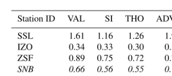
Table 4.Standard deviations of the remainder components by STL over 2010 to 2015, except for SNB. Data at SNB were decomposed over 2012 to 2015 due to missing data from 2010 to 2011 and thus shown in italic font.
Station ID VAL SI THO ADVS
SSL 1.61 1.16 1.26 1.99
IZO 0.34 0.33 0.30 0.30
ZSF 0.89 0.75 0.72 0.73
SNB 0.66 0.56 0.55 0.70
JFJ 0.56 0.45 0.48 0.47
3.4 Correlation analysis
As mentioned above, data selection is defined here as an ap-proach of extracting a group of data to be the best repre-sentative for the lower free troposphere. Consequently, the selected CO2 datasets should have properties that are well
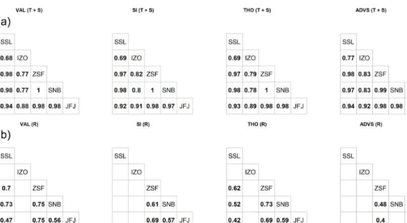
Figure 6.Pearson’s correlation matrices of combinations of trend and seasonal components (T+S,a), and only remainder components (R,b) at stations SSL, IZO, ZSF, SNB, and JFJ by different selection methods. Correlations with no significant coefficients at the 0.05 significance level were left blank.
with selected data irrespective of the selection method, es-pecially between the three Alpine stations (ZSF, SNB, and JFJ). This evaluation shows a similar result to the method presented by Sepúlveda et al. (2014) for identifying base-line conditions based on the correlation between distant mea-suring stations. Pairs including IZO after data selection by ADVS show a notable increase in the correlation coefficients, meaning better coherence between the reference station IZO and the others.
Conversely, when selecting representative data more effec-tively, the results should contain less local and regional influ-ences. Therefore, we compared the remainder components derived from STL pairwise to check whether the Pearson correlation coefficients decreased after data selection (see Fig. 6b). The number of insignificant correlations between the station pairings is the greatest for ADVS. For the only two coefficients significant at the 0.05 significance level (ZSF-SNB and ZSF-JFJ), they drop largely from 0.75 to 0.48, and from 0.75 to 0.40, respectively, which cannot be observed by the other selection methods. This means that by ADVS the combination of trend and seasonal components correlate best and the remaining unselected data have the lowest correlation among the methods. If these two criteria are used to separate the representative part of the data from the unrepresentative part, the ADVS method produces the best results.
4 Conclusions and outlook
We presented the novel statistical ADVS method for se-lecting representative baseline data for CO2 measurements
at elevated GAW mountain stations. For assessment of the
data selection procedure, we applied the method to six CO2
datasets measured at GAW mountain stations in the Euro-pean Alps. The ADVS resulted in an increasing number of percentages of selected data representing the background conditions with growing altitude of continental measurement sites, which is reasonable due to the underlying atmospheric dynamics. For comparison, three well-known statistical data selection methods were applied to the same datasets and most methods yielded similar increasing percentages with growing altitude. Among all the methods, ADVS is the most restric-tive in terms of the number of selected data in the overall datasets.
In addition, we applied the time series decomposition method STL to all datasets before and after data selec-tion. All statistical data selection methods resulted in the same annual trend within the 95 % confidence interval of the datasets before selection, while the seasonal signal var-ied substantially with smaller seasonal amplitudes and de-layed occurrences of seasonal maxima. We also presented an additional assessment of ADVS compared with the other sta-tistical data selection methods based on correlation analysis. For the combination of trend and seasonal components by STL, higher correlation coefficients between stations were found with ADVS data selection than SI and THO. Inversely, ADVS resulted in lower correlation coefficients in the re-mainder components than the other methods. Both indicate a better performance of selecting baseline data by ADVS.
The presented method is useful for data selection of at-mospheric CO2 data representative of the lower free
automatically. The method can also be applied to histori-cal datasets. The results provide evidence that the proposed ADVS method confers the possibility of selecting data that are representative of CO2concentrations of a larger area of
the lower free troposphere. This is an elementary prerequi-site for application of the method to a larger number of dif-ferent stations and an essential step towards generalization. It directly supports the objective of GAW to extrapolate from a set of point measurements from single stations to a larger representative area or region in the lower free troposphere (WMO, 2017). In future, there is a need to test whether such results could be used for additional applications, such as ground calibration of satellite measurements. Finally, it would be very interesting to test as a next step whether this presented method is applicable to stations in other regions and on other continents. Moreover, the issue of whether and how to include coastal stations in a systematic and practi-cally generalizable approach for selecting representative data at GAW stations will be a particular concern.
Data availability. Hourly CO2 data can be downloaded from
WMO’s World Data Centre for Greenhouse Gases (http:// ds.data.jma.go.jp/gmd/wdcgg/cgi-bin/wdcgg/catalogue.cgi; last ac-cess: 15 March 2018), data with higher resolution can be requested from the station data providers.
Supplement. The supplement related to this article is available online at: https://doi.org/10.5194/amt-11-1501-2018-supplement.
Competing interests. The authors declare that they have no conflict of interest.
Acknowledgements. This work was supported by a scholar-ship from China Scholarscholar-ship Council (CSC) under grant CSC No. 201508080110. This work was supported by a MICMoR Fellowship through KIT/IMK-IFU to Ye Yuan. This work was supported by the German Research Foundation (DFG) and the Technical University of Munich (TUM) in the framework of the Open Access Publishing Program. The CO2 measurements
at Zugspitze and Schauinsland were supported by the German Environment Agency (UBA). We thank Markus Wallasch for providing CO2data obtained at Schauinsland and Ralf Sohmer for
technical support. The CO2 measurements at Hohenpeissenberg
were conducted by the German Meteorological Service within the ICOS Atmospheric Station Network. The CO2 measurements at Jungfraujoch were supported by the Swiss Federal Office for the Environment, ICOS-Switzerland, and the International Foundation High Alpine Research Stations Jungfraujoch and Gornergrat. Martin Steinbacher acknowledges funding from the GAW Quality Assurance/Science Activity Centre Switzerland (QA/SAC-CH), which is supported by MeteoSwiss and Empa. The Izaña (IZO) CO2 measurements were performed within the GAW Program
at the Izaña Atmospheric Research Center, financed by AEMET.
Finally, we also thank Wolfgang Spangl from the Austrian Envi-ronment Agency (UBA-At) for providing CO2 data obtained at
Sonnblick.
This work was supported by the German Research Foundation (DFG) and the Technische Universität München within the funding programme Open Access Publishing.
Edited by: Dominik Brunner
Reviewed by: Jooil Kim and one anonymous referee
References
Bacastow, R. B., Keeling, C. D., and Whorf, T. P.: Seasonal Am-plitude Increase in Atmospheric CO2 Concentration at Mauna
Loa, Hawaii, 1959–1982, J. Geophys. Res., 90, 10529–10540, https://doi.org/10.1029/JD090iD06p10529, 1985.
Balzani Lööv, J. M., Henne, S., Legreid, G., Staehelin, J., Reimann, S., Prévôt, A. S. H., Steinbacher, M., and Vollmer, M. K.: Esti-mation of background concentrations of trace gases at the Swiss Alpine site Jungfraujoch (3580 m a.s.l.), J. Geophys. Res., 113, D22305, https://doi.org/10.1029/2007JD009751, 2008. Birmili, W., Ries, L., Sohmer, R., Anastou, A., Sonntag, A., König,
K., and Levin, I.: Feine und ultrafeine Aerosolpartikeln an der GAW-Station Schneefernerhaus/Zugspitze, Gefahrst. Reinhalt. L., 69, 31–35, 2009.
Brailsford, G. W., Stephens, B. B., Gomez, A. J., Riedel, K., Mikaloff Fletcher, S. E., Nichol, S. E., and Manning, M. R.: Long-term continuous atmospheric CO2measurements at
Bar-ing Head, New Zealand, Atmos. Meas. Tech., 5, 3109–3117, https://doi.org/10.5194/amt-5-3109-2012, 2012.
Brooks, B.-G. J., Desai, A. R., Stephens, B. B., Bowling, D. R., Burns, S. P., Watt, A. S., Heck, S. L., and Sweeney, C.: Assess-ing filterAssess-ing of mountaintop CO2mole fractions for application
to inverse models of biosphere-atmosphere carbon exchange, At-mos. Chem. Phys., 12, 2099–2115, https://doi.org/10.5194/acp-12-2099-2012, 2012.
Calvert, J. G.: Glossary of atmospheric
chem-istry terms, Pure Appl. Chem., 62, 2167–2219, https://doi.org/10.1351/pac199062112167, 1990.
Carnuth, W. and Trickl, T.: Transport studies with the IFU three-wavelength aerosol lidar during the VOTALP Mesolcina experiment, Atmos. Environ., 34, 1425–1434, https://doi.org/10.1016/S1352-2310(99)00423-9, 2000. Carnuth, W., Kempfer, U., and Trickl, T.: Highlights of the
tropo-spheric lidar studies at IFU within the TOR project, Tellus B, 54, 163–185, https://doi.org/10.1034/j.1600-0889.2002.00245.x, 2002.
Carslaw, D. C.: On the changing seasonal cycles and trends of ozone at Mace Head, Ireland, Atmos. Chem. Phys., 5, 3441– 3450, https://doi.org/10.5194/acp-5-3441-2005, 2005.
Sta-tions Using Radon-222, Aerosol Air Qual. Res., 16, 885–899, https://doi.org/10.4209/aaqr.2015.06.0391, 2016.
Cleveland, R. B., Cleveland, W. S., McRae, J. E., and Terpenning, I.: STL: A seasonal-trend decomposition procedure based on Loess, J. Off. Stat., 6, 3–73, 1990.
Cleveland, W. S.: Robust locally weighted regression and smoothing scatterplots, J. Am. Stat. Assoc., 74, 829–836, https://doi.org/10.1080/01621459.1979.10481038, 1979. Cleveland, W. S., Freeny, A. E., and Graedel, T. E.: The
Seasonal Component of Atmospheric CO2: Information
From New Approaches to the Decomposition of Sea-sonal Time Series, J. Geophys. Res., 88, 10934–10946, https://doi.org/10.1029/JC088iC15p10934, 1983.
Cui, J., Pandey Deolal, S., Sprenger, M., Henne, S., Staehelin, J., Steinbacher, M., and Nédélec, P.: Free tropospheric ozone changes over Europe as observed at Jungfraujoch (1990–2008): An analysis based on backward trajectories, J. Geophys. Res., 116, D10304, https://doi.org/10.1029/2010JD015154, 2011. Elliott, W. P. (Ed.): The Statistical treatment of CO2data records,
NOAA Technical Memorandum ERL ARL, 173, U.S. Dept. of Commerce, National Oceanic and Atmospheric Administration, Environmental Research Laboratories, Silver Spring, Md., USA, 131 pp., 1989.
Fang, S. X., Tans, P. P., Steinbacher, M., Zhou, L. X., and Luan, T.: Comparison of the regional CO2mole fraction filtering
ap-proaches at a WMO/GAW regional station in China, Atmos. Meas. Tech., 8, 5301–5313, https://doi.org/10.5194/amt-8-5301-2015, 2015.
Forrer, J., Rüttimann, R., Schneiter, D., Fischer, A., Buch-mann, B., and Hofer, P.: Variability of trace gases at the high-Alpine site Jungfraujoch caused by meteorologi-cal transport processes, J. Geophys. Res., 105, 12241–12251, https://doi.org/10.1029/1999JD901178, 2000.
Gilge, S., Plass-Duelmer, C., Fricke, W., Kaiser, A., Ries, L., Buch-mann, B., and Steinbacher, M.: Ozone, carbon monoxide and nitrogen oxides time series at four alpine GAW mountain sta-tions in central Europe, Atmos. Chem. Phys., 10, 12295–12316, https://doi.org/10.5194/acp-10-12295-2010, 2010.
Gomez-Pelaez, A. J., Ramos, R., Cuevas, E., and Gomez-Trueba, V.: 25 years of continuous CO2 and CH4 measurements at
Izaña Global GAW mountain station: annual cycles and interan-nual trends, in: Proceedings of the Symposium on Atmospheric Chemistry and Physics at Mountain Sites (ACP Symposium 2010), 8–10 June 2010, Interlaken, Switzerland, 157–159, 2010. Gomez-Pelaez, A. J., Ramos, R., Gomez-Trueba, V., Novelli, P. C., and Campo-Hernandez, R.: A statistical approach to quan-tify uncertainty in carbon monoxide measurements at the Izaña global GAW station: 2008–2011, Atmos. Meas. Tech., 6, 787– 799, https://doi.org/10.5194/amt-6-787-2013, 2013.
Henne, S., Brunner, D., Folini, D., Solberg, S., Klausen, J., and Buchmann, B.: Assessment of parameters describing repre-sentativeness of air quality in-situ measurement sites, Atmos. Chem. Phys., 10, 3561–3581, https://doi.org/10.5194/acp-10-3561-2010, 2010.
Hernández-Paniagua, I. Y., Lowry, D., Clemitshaw, K. C., Fisher, R. E., France, J. L., Lanoisellé, M., Ramonet, M., and Nisbet, E. G.: Diurnal, seasonal, and annual trends in atmospheric CO2
at southwest London during 2000–2012: Wind sector analysis
and comparison with Mace Head, Ireland, Atmos. Environ., 105, 138–147, https://doi.org/10.1016/j.atmosenv.2015.01.021, 2015. Herrmann, E., Weingartner, E., Henne, S., Vuilleumier, L., Bukowiecki, N., Steinbacher, Coen, F., Collaud Conen, M., Ham-mer, E., Jurányi, Z., Baltensperger, U., and Gysel, M.: Analy-sis of long-term aerosol size distribution data from Jungfraujoch with emphasis on free tropospheric conditions, cloud influence, and air mass transport, J. Geophys. Res.-Atmos., 120, 9459– 9480, https://doi.org/10.1002/2015JD023660, 2015.
Kaiser, A., Scheifinger, H., Spangl, W., Weiss, A., Gilge, S., Fricke, W., Ries, L., Cemas, D., and Jesenovec, B.: Transport of nitrogen oxides, carbon monoxide and ozone to the Alpine Global Atmosphere Watch stations Jungfraujoch (Switzerland), Zugspitze and Hohenpeissenberg (Germany), Sonnblick (Aus-tria) and Mt. Krvavec (Slovenia), Atmos. Environ., 41, 9273– 9287, https://doi.org/10.1016/j.atmosenv.2007.09.027, 2007. Keeling, C. D.: The Concentration and Isotopic Abundances
of Carbon Dioxide in the Atmosphere, Tellus, 12, 200–203, https://doi.org/10.1111/j.2153-3490.1960.tb01300.x, 1960. Locher, R. and Ruckstuhl, A.: IDPmisc: Utilities of Institute of
Data Analyses and Process Design, available at: https://CRAN. R-project.org/package=IDPmisc (last access: 28 August 2017), 2012.
Lowe, D. C., Guenther, P. R., and Keeling, C. D.: The con-centration of atmospheric carbon dioxide at Baring Head, New Zealand, Tellus, 31, 58–67, https://doi.org/10.1111/j.2153-3490.1979.tb00882.x, 1979.
Massen, F. and Beck, E.-G.: Accurate Estimation of CO2 Back-ground Level from Near Ground Measurements at Non-Mixed Environments, in: The Economic, Social and Political Elements of Climate Change, edited by: Leal Filho, W., Climate Change Management, Springer Berlin Heidelberg, Berlin, Heidelberg, Germany, 509–522, 2011.
Pales, J. C. and Keeling, C. D.: The Concentration of Atmospheric Carbon Dioxide in Hawaii, J. Geophys. Res., 70, 6053–6076, https://doi.org/10.1029/JZ070i024p06053, 1965.
Parrish, D. D., Law, K. S., Staehelin, J., Derwent, R., Cooper, O. R., Tanimoto, H., Volz-Thomas, A., Gilge, S., Scheel, H.-E., Steinbacher, M., and Chan, E.: Long-term changes in lower tropospheric baseline ozone concentrations at north-ern mid-latitudes, Atmos. Chem. Phys., 12, 11485–11504, https://doi.org/10.5194/acp-12-11485-2012, 2012.
Peterson, J. T., Komhyr, W. D., Harris, T. B., and Waterman, L. S.: Atmospheric carbon dioxide measurements at Barrow, Alaska, 1973–1979, Tellus, 34, 166–175, https://doi.org/10.1111/j.2153-3490.1982.tb01804.x, 1982.
Pickers, P. A. and Manning, A. C.: Investigating bias in the applica-tion of curve fitting programs to atmospheric time series, Atmos. Meas. Tech., 8, 1469–1489, https://doi.org/10.5194/amt-8-1469-2015, 2015.
R Core Team: R: A Language and Environment for Statistical Com-puting, Vienna, Austria, available at: https://www.R-project.org/, last access: 28 August 2017.
Reiter, R., Sladkovic, R., and Kanter, H.-J.: Concentration of trace gases in the lower troposphere, simultaneously recorded at neigh-boring mountain stations, Meteorol. Atmos. Phys., 35, 187–200, https://doi.org/10.1007/BF01041811, 1986.
station for clouds and turbulence, Atmos. Meas. Tech., 8, 3209– 3218, https://doi.org/10.5194/amt-8-3209-2015, 2015.
Ruckstuhl, A. F., Henne, S., Reimann, S., Steinbacher, M., Vollmer, M. K., O’Doherty, S., Buchmann, B., and Hueglin, C.: Ro-bust extraction of baseline signal of atmospheric trace species using local regression, Atmos. Meas. Tech., 5, 2613–2624, https://doi.org/10.5194/amt-5-2613-2012, 2012.
Satar, E., Berhanu, T. A., Brunner, D., Henne, S., and Leuenberger, M.: Continuous CO2/CH4/CO measurements (2012–2014) at
Beromünster tall tower station in Switzerland, Biogeosciences, 13, 2623–2635, https://doi.org/10.5194/bg-13-2623-2016, 2016. Schibig, M. F., Steinbacher, M., Buchmann, B., van der Laan-Luijkx, I. T., van der Laan, S., Ranjan, S., and Leuenberger, M. C.: Comparison of continuous in situ CO2observations at
Jungfraujoch using two different measurement techniques, At-mos. Meas. Tech., 8, 57–68, https://doi.org/10.5194/amt-8-57-2015, 2015.
Schmidt, M., Graul, R., Sartorius, H., and Levin, I.: The Schauinsland CO2 record: 30 years of continental observa-tions and their implicaobserva-tions for the variability of the Eu-ropean CO2 budget, J. Geophys. Res.-Atmos., 108, 4619,
https://doi.org/10.1029/2002JD003085, 2003.
Sepúlveda, E., Schneider, M., Hase, F., Barthlott, S., Dubravica, D., García, O. E., Gomez-Pelaez, A., González, Y., Guerra, J. C., Gisi, M., Kohlhepp, R., Dohe, S., Blumenstock, T., Strong, K., Weaver, D., Palm, M., Sadeghi, A., Deutscher, N. M., Warneke, T., Notholt, J., Jones, N., Griffith, D. W. T., Smale, D., Brails-ford, G. W., Robinson, J., Meinhardt, F., Steinbacher, M., Aalto, T., and Worthy, D.: Tropospheric CH4 signals as observed by
NDACC FTIR at globally distributed sites and comparison to GAW surface in situ measurements, Atmos. Meas. Tech., 7, 2337–2360, https://doi.org/10.5194/amt-7-2337-2014, 2014.
Sirignano, C., Neubert, R. E. M., Rödenbeck, C., and Meijer, H. A. J.: Atmospheric oxygen and carbon dioxide observations from two European coastal stations 2000–2005: continental influence, trend changes and APO climatology, Atmos. Chem. Phys., 10, 1599–1615, https://doi.org/10.5194/acp-10-1599-2010, 2010. Stephens, B. B., Brailsford, G. W., Gomez, A. J., Riedel, K.,
Mikaloff Fletcher, S. E., Nichol, S., and Manning, M.: Anal-ysis of a 39-year continuous atmospheric CO2 record from
Baring Head, New Zealand, Biogeosciences, 10, 2683–2697, https://doi.org/10.5194/bg-10-2683-2013, 2013.
Thoning, K. W., Tans, P. P., and Komhyr, W. D.: Atmospheric Carbon Dioxide at Mauna Loa Observatory: 2. Analysis of the NOAA GMCC Data, 1974–1985, J. Geophys. Res., 94, 8549– 8565, https://doi.org/10.1029/JD094iD06p08549, 1989. Uglietti, C., Leuenberger, M., and Brunner, D.: European source
and sink areas of CO2 retrieved from Lagrangian
trans-port model interpretation of combined O2 and CO2
measure-ments at the high alpine research station Jungfraujoch, Atmos. Chem. Phys., 11, 8017–8036, https://doi.org/10.5194/acp-11-8017-2011, 2011.
WMO: WMO Global Atmosphere Watch (GAW) Implementation Plan: 2016–2023, Geneva, Switzerland, 81 pp., 2017.
Zeileis, A. and Grothendieck, G.: zoo: S3 Infrastructure for Regular and Irregular Time Series, J. Stat. Soft., 14, 1–27, https://doi.org/10.18637/jss.v014.i06, 2005.