CFD SIMULATIONS AND FLOW ANALYSIS THROUGH A T-JUNCTION PIPE

(1)

ANALYSIS THROUGH A T-JUNCTION

PIPE

Mohammed Abdulwahhab

a

, Prof. Niranjan Kumar Injeti

b

, Ass. Prof. Sadoun Fahad Dakhil

c

a: Research Scholar, Department of Marin Engineering, Andhra University, AP, India. b: Department of Marin Engineering, Andhra University, AP, India.

c: Department of Fuel& Energy, Basrah Technical College, Iraq.

ABSTRACT

An extensive three dimensional numerical parametric investigation of the turbulent flow in 90 ̊T-junctions with

sharp corners is underway aimed at quantifying the energy losses and the size and strength of the re-circulating region in the zone close the connecting zone i.e. connect branch with main pipes. Pressure drop and friction coefficient are solved from Navier-Stock equations into Cartesian coordinates by using finite volume method with both simple algorithm and upwind schemes.

The simulations carried out for an inlet pipe Reynolds numbers of 36000, for flow rate ratios from 0% to 100% (ratio between the flow rates in the branch and outlet pipe). Results show high effect of the flow rate ratio on the pressure loss and then the outlet flow rate. At Re (36000) and q2/q3 (50%) the axial outlet flow rate reached

maximum value of about (0.00146029 m3/s).

Keywords: T-junction,turbulent flow, sharp edge, flow rate ratio.

1. INTORDUCTION

Pipe networks are very common in industries, where fluid or gases to be transported from one location to the other. The pressure loss may vary depending on the type of components coming across in the network, material of the pipe, and the fluid that is being transported through the network. The placement of valves, pumps and turbines is important to overcome the pressure loss caused by other components in the network. This is one of the important reasons why this study was conducted.

In this work we have concentrated our attention to a very small and common component of pipe network: T-junction is a very common component in pipe networks, mainly used to distribute (diverge) the flow from main pipe to several branching pipes and to accumulate (converge) flows from many pipes to a single main pipe.

Flows in T-junctions are highly complex and three-dimensional, therefore requiring experimental or numerical treatment. The former requires a significant amount of effort and there is much understanding to be gained from numerical simulations. From the numerical perspective this turbulent flow is also quite challenging because it combines streamline curvature, turbulence anisotropy and re-circulating regions.

Early experimental work on this subject started in Munich with Vogel [12] and continued with Gardel [3] as reviewed in detail by Maia [7]. Numerical investigations on T-junction flows are scarce in the literature: Sierra-Espinoza and Bates [11] used various turbulence models and concluded that although the k-ε, RNG and RSM turbulence models predicted the mean flow qualitatively. Miller (1990) [8] states that the cause of major energy loss for T and Y junctions is due to the combination and division of flows, which arise from separation and subsequent turbulent mixing.

(2)

2. PROBLEM SPECIFICATION

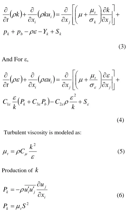
Figure (1) shows a schematic representation of the flow distribution through pipe and a general physical setup.

Fluid enters the pipe at one end and exit from the other in axial directionand this is merged with fluid that is coming from the upper one inradial direction.

To analyze the fundamental system properties and flow patterns, a simplified flow model was employed in this study. It represents the pipe flow situation as the flow in a straight pipe i.e. main pipe in horizontal direction with one vertical pipe i.e. branch pipe which is connected with the main pipe by an angle of 90 ̊.

The modeled flow distribution system considered for this purpose is of diameter D1 as 1 inch for horizontal pipe or

the main pipe and the vertical pipe considered D2 as 1 inch i.e. branch pipe. The area ratio between the main pipe

and branch pipe considered as A1/A2=1.

Water enters at a uniform temperature at T= 25 ̊C, constant velocity for inlet 1 at first stage with different values of velocities for inlet 2, and the second stage is vice versa. In this work, we are investigating the following range of the flow rates; 0<q<1 corresponding to the velocity ratio of branch or radial pipe to outlet pipe in axial direction is (v2/v3).

3. GOVERNING EQUATIONS

The equations to be solved for incompressible flow are the conservation of mass Eq. (1) and momentum Eq. (2) in Cartesian coordinate.



0 



i i

x

U

(1)

















































j i i j j i j i j i j i

u

x

U

x

U

x

p

x

U

t

U







(2)

Where: u is main axial velocity and U is bulk velocity.

The above two equations (1) and (2) are the Navier-Stokes equations. Many researchers have attempted to solve these equations but the computational complexity involved has not allowed many but arrived at some solutions. Navier-Stokes equation can be solved numerically by using finite volume method, but the solutions are obtained only after making some assumptions and some of them are not stable at high Reynolds number [5].

The

k





model is one of the most commonly used turbulence models. It includes two transport equations to represent the turbulent properties of the flow. The first transported variable is turbulent kinetic energy

k

. The second transported variable in this case is the turbulent dissipation



. These variables determine the scale of the turbulence and energy in the turbulence. The

k





model is most commonly used to describe the behavior of the turbulent flow.





u

_i

u

_j represent the last term of equation (2) as a time average eddy shear stress in the momentum equation, where the molecular diffusion shear stress

i

x

u





is augmented by this shear stress and important role

(3)

k k b k j k j i

S

Y

p

x

t

























(3)

And For

ε

,

 











   













S

k

C

P

C

P

k

C

x

u

x

t

b k j t j i i













































2 2 3 1

(4)

Turbulent viscosity is modeled as:







t



C

_

k

2

(5)

Production of

k

2

S

P

x

u

P

t k i j j i k















(6)

S

is the modulus of the mean rate-of-strain tensor, defined as:

Sij

S



2

_ij (7)

Realizable

k

-epsilon model and RNG

k

-epsilon model are some other variation of

k

-epsilon model.

k

-epsilon model has solution in some special cases.

k

-epsilon model is only useful in regions with turbulent, high Reynolds number flows. The equations contain four adjustable constants. The standard

k





model employs values for the constants that are arrived at by comprehensive data fitting for a wide range of turbulent flows:

σ

k

σ

ε

C

1ε

C

2ε

C

µ

1.00 1.30 1.44 1.92 0.09

(4)

3. FLOW PARAMETERS

3.1. FLOW GEOMETRY

The T-junction was drawn with the Cartesian coordinate system and the notationis presented in figure (1). From figure (1) the author has assumed that the diameter of pipe was 1 inch (0.0254 m) everywhere. The length of the entrance pipes at upstream 1 is -10D to -0.5D and upstream 2 is 0D to 10D and for the downstream it is 0.5D to 10D. The direction of main flow is x direction as mentioned in the diagram. The origin of the coordinate system is located at the center of the pipe as shown in figure (1). The T-piece looks very similar and with sharp edges.

The flow configuration is that of a convergence flow in a 90 ̊ T-junction with sharp corners with equal bifurcating pipes and different flow rates to show the effect of Reynolds number (flow rate ratio) on the outlet flow. By numbering the flow paths as legs 1, 2, and 3 (leg 3 carrying the total flow) as shown in figure (1).

3.2. SIMULATION PARAMETERS

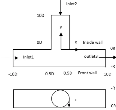
The fluid used in the simulations is water with constant density of 998.2 kg/m3 and dynamic viscosity of 0.001 kg/m s. The fluid is assumed as Incompressible flow. The boundary conditions were set as a mass flow at the two inlets and as pressure at the outlet. The two inlets depend on the value of velocities and the flow rate ratio between the inlet 2 and outlet 3. The inlet boundary conditions are normal to surface area of inlet 1 and inlet 2. The velocity at the inlet pipes (upstream) is fully developed. It is assumed that no-slip boundary conditions at all the walls. As the flow is axisymmetric the complete geometry is taken into consideration. Figure (2) is the unstructured computational grids (Tetrahedral 42929 & Prism 33450 cells), the mesh consist from 26113 nodes and 76379 elements with five boundary layers. The calculations were carried out with commercial finite volume code ANSYS CFX 13 using a second order scheme.

Figure (1) Schematic representation of the T-Junction

outlet3

0R y

x

z

Inlet2

Inlet1

10D

0.5D ‐0.5D ‐10D

0D 10D

‐R

0R ‐R

Inside wall

(5)

Figure (2) The unstructured mesh for T-junction

4. CFD SIMULATIONS AND RESULTS

According to the flow configuration of figure (1), the energy equations for the flow paths are given by

13 2 3 3 3 3 2 1 1 1 1 2 3 3 3 2 1 1 1

2

1

2

1 











U

D

L

f

U

D

L

f

U









(8) 23 2 3 3 3 3 2 2 2 2 2 2 3 3 3 2 2 2 2

2

1

2

1 











U

D

L

f

U

D

L

f

U









(9)

for the straight and branched flows, respectively. The subscripts 1, 2 and 3 refer to the inlet pipe, branch pipe and the straight outlet pipe, respectively. The energy shape factors (



) are taken to be 1 [2], the usual engineering practice in calculations when the flow is turbulent. From the pressure calculates taken along the straight pipes, in regions of fully developed flow, the values of the Darcy friction factors were determined for each pipe. The pressure losses in the tee were subsequently evaluated from equations (8) and (9). The corresponding local loss coefficients are defined as 2 3 13 13

2

1 U

km







(10)

2 3 23 23

2

1 U

km







(11)

It is important to note at first stage that the inlet Reynolds numbers (Re1) is fixed as 36000 and change to the inlet Reynolds numbers (Re2) from 6.5x103 to 6.34x105, for the second stage the inlet Reynolds numbers (Re1) is change from 6.5x103 to 6.34x105 and fixed the inlet Reynolds numbers (Re2) as 36000. At high Reynolds number flows where the loss coefficients are already independent of Reynolds number.

Figure (3) represents the pressure contour at midsection of the sketch for q=50%, V1 & V2= 1.42 m/s for each one.

(6)

zone near branch pipe has negative value of pressure due to swirls that happened due to change in the direction of the flow. Finally the pressure drop at downstream, then the velocity become high at outlet.

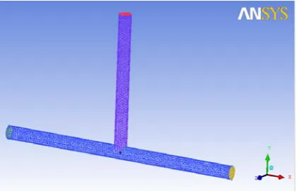
Figure (4) represents the pressure loss coefficient km13 for straight pipe (from inlet 1 to outlet 3) at Re=36000 and

Figure (5) at different Re as mentioned above. It is observed that there are few differences in the values of km13 in

two cases.

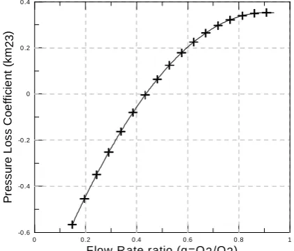
Figure (6) represents the pressure loss coefficient km23 for branch pipe (from inlet 2 to outlet 3) at Re=36000 and

figure (7) at different Reynolds number as mentioned above. It is observed that there are few differences in the values of km23 in two cases.

Figures (8) and (9) depicts the comparison of our results with the available literature, it is clear that is not reasonably well considering the differences in Reynolds number with literature, variation in the geometry, the inlet flow conditions, and the material is different because the later used air. The values of km13 for the present work are less

than Miller (1990) but q from 0 to 0.3 we notice values of km13 are greater than the results of Miller [8].

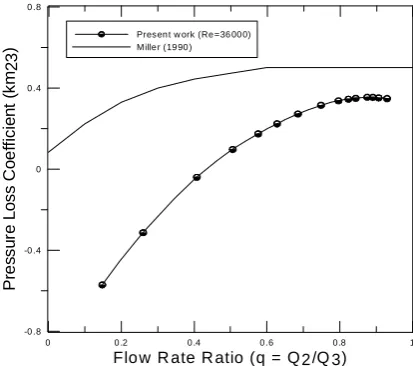
Figures (10) and (11) depicts the comparison of results with Miller (1990) [8] for the values of km23 showed the

same reasons as mentioned above.

From numerical results, at Reynolds number of 36000 and a flow rate ratio of 50%, the values of km13 and km23 are

equal to 0.1358 and 0.081, respectively. .

Figure ( 3) The Pressure Contour, at q=50%, V1=1.42 m/s & V2=1.42 m/s.

0 0.2 0.4 0 .6 0 .8 1

F low R ate Ratio (q=Q 2/Q3) -0 .1

0 0 .1 0 .2

P

re

ssu

re

L

o

ss

C

o

e

ffi

c

ie

n

t

(km

13

)

(7)

0 0 .2 0 .4 0 .6 0 .8 1 F low R ate R atio (q =Q 2/Q3)

-0 .4 -0 .2 0 0 .2

P

re

s

u

re

Lo

ss

Co

ef

fi

c

ie

n

t

(km

13

Figure (5) The pressure loss coefficient for straight pipe, at different Re.

0 0 .2 0 .4 0 .6 0 .8 1

F low R ate R atio (q =Q 2/Q3) -1 .2

-0 .8 -0 .4 0 0 .4 0 .8

P

re

s

u

re

Lo

ss

C

o

e

ff

ic

ien

t

(km

23

)

Figure (6) The pressure loss coefficient for branch pipe, Re=36000.

0 0.2 0.4 0 .6 0 .8 1

Flow R ate ratio (q=Q2/Q3) -0 .6

-0 .4 -0 .2 0 0 .2 0 .4

P

re

s

su

re

Lo

ss

C

o

e

ff

ic

ie

n

t

(k

m23

)

(8)

0 0 .2 0 .4 0 .6 0 .8 1 Flow Ra te R a tio (q = Q2/Q 3)

-0 .8 -0 .4 0 0 .4 0 .8 1 .2

P

re

s

u

re

Lo

ss

co

e

ff

ic

ie

n

t

(k

m13

) Pre se nt W ork (Re =36 00 0)Miller (1 99 0)

Figure (8) Comparison the variation of the pressure loss coefficient for straight pipe.

0 0 .2 0 .4 0 .6 0 .8 1

Flow Ra te R a tio (q = Q 2 /Q 3) -0 .8

-0 .4 0 0 .4 0 .8 1 .2

P

re

s

su

re

L

o

ss

C

o

ef

fi

c

ie

n

t

(k

m13

) P re se nt w o rkM iller (1 99 0)

Figure (9) Comparison of the variation of the pressure loss coefficient for straight pipe, at various Re.

0 0 .2 0 .4 0 .6 0 .8 1

Flow R ate R atio (q = Q 2/Q 3) -0 .8

-0 .4 0 0 .4 0 .8

P

res

su

re

L

o

s

C

o

ef

fi

c

ie

n

t

(km

23

)

Presen t w ork (Re =36 00 0) Mille r (19 90 )

(9)

0 0 .2 0 .4 0 .6 0 .8 1

F lo w R a te ra tio ( q = Q 2 /Q 3 )

-1 .2 -0 .8 -0 .4 0 0 .4

P

re

s

u

re

L

o

s

C

o

ef

fi

c

ien

t

(k

m23

Figure (11) Comparison of the variation of the pressure loss coefficient for branch pipe, at various Re.

4.1. Velocity Profiles

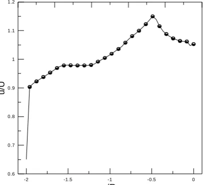
We start by presenting the mean velocity in the horizontal plane x-y of the upstream inlet 1 for main pipe and

inlet 2 for branch pipe. In figure (12), the inlet main pipe u is the streamline velocity and the inlet branch pipe the velocity –v. The velocity profile in each inlet at each cross section is fully developed. On approaching the beginning of the bifurcation (-0.5D) for main pipe and (0D) for branch pipe, the flow is merging in the downstream of the main pipe. The flow at both inlets is well developed upstream the bifurcation.

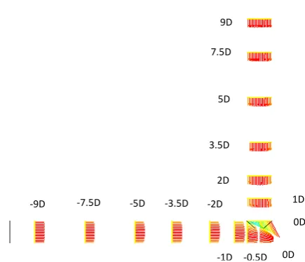
Figure (13) depicts the change in the velocity profiles in the downstream from cross section (0D) to the outlet (10D). It is very clear that the circulation bubble becomes wider and starting from (0D) cross section. These re-circulating are concentrating near the upper wall of the downstream exactly at the zone near bifurcation, also that the fluid is moving away from the wall, and continuity requires that an inflow into the wall region must take place.

Figure (12) Vector plot of the mean velocity in the horizontal plane x-y of the upstream bifurcation of the sharp-edge for Re=36000 and q=50%.

Figure (13) Vector plot of the mean velocity in the horizontal plane x-y of the downstream bifurcation of the sharp-edge for Re=36000 and q=50%.

‐9D ‐7.5D ‐5D ‐3.5D ‐2D

9D

7.5D

5D

3.5D

2D

0D

1D

‐1D ‐0.5D 0D

9.5D 3D

1.5D 0.5D

(10)

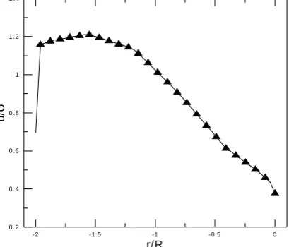
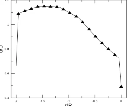
Figures (14-23) represents the radial profile of the longitudinal velocity at various cross sections along the downstream of the outlet pipe with sharp edge, Re=36000 and flow rate ratio 50%. In the downstream from entrance to exit the velocity profiles become quickly distorted due to the flow coming from the branch pipe and developed the re-circulation near the wall. Flow recirculation in the outlet pipe is noticed at 1.5D and 2.5D. The fluid is already accelerating from the center of the pipe towards front wall (-R) and further towards the outer wall as shown in figure 1, but at 7.5D the profile is still distorted.

Figure (23) represents the radial velocity profile at cross section 9.5D. It is noticed that the peak velocity increases from the center of the pipe towards the front wall (-R). But the velocity near the inside wall (0R) is still less than the velocity close to the front wall, from this it is observed that the velocity is close to fully developed because still at the entry of the main pipe downstream where entrance length



e



10 D

.

-2 -1.5 -1 -0.5 0

r/R

0.6 0.7 0.8 0.9 1 1.1 1.2

u/

U

Figure (14) Radial profile of the longitudinal velocity in the outlet pipe of the sharp edge for Re=36000 and Q2/Q3=50% at 0.5D downstream.

-2 -1.5 -1 -0.5 0

r/R

0.2 0.4 0.6 0.8 1 1.2

u/

U

(11)

-2 -1 .5 -1 -0 .5 0 r/R

0 0 .4 0 .8 1 .2

u/

U

-2 -1 .5 -1 -0 .5 0

r/R 0

0 .4 0 .8 1 .2

u/

U

-2 -1 .5 -1 -0 .5 0

r/R 0 .2

0 .4 0 .6 0 .8 1 1 .2 1 .4

u/

U

(12)

-2 -1 .5 -1 -0 .5 0 r/R

0 .4 0 .6 0 .8 1 1 .2

u/

U

-2 -1 .5 - 1 -0 .5 0

r/R

0 .4 0 .6 0 .8 1 1 .2

u/

U

-2 -1 .5 - 1 -0 .5 0

r/R

0 .4 0 .6 0 .8 1 1 .2

u/

U

(13)

-2 -1 .5 -1 -0 .5 0 r/R

0 .4 0 .6 0 .8 1

u/

U

Figure (22) Radial profile of the longitudinal velocity in the outlet pipe of the sharp edge for Re=36000 and Q2/Q3=50% at 8.5D downstream.

-2 -1 .5 -1 -0 .5 0

r/R 0 .4

0 .6 0 .8 1 1 .2

u/

U

Figure (23) Radial profile of the longitudinal velocity in the outlet pipe of the sharp edge for Re=36000 and Q2/Q3=50% at 9.5D downstream.

Figures (24) and (25) represent the horizontal profile of the longitudinal velocity in the outlet pipe with the sharp edge where Re=36000 and flow rate ratio q=50% for six locations at the downstream. It is noticed that the behavior of the velocity profiles are different from radial profiles. This is not just because of the shape but it different because of the velocity values. At cross section 1.5D the maximum value of velocities are near the walls but at the center of the pipe the velocity values are minimum. At cross section 2.5D the behavior of the velocity profile is the same as previous section but the values of velocity are decreased. At cross section 5D the behavior of profile initiated changes. The values of the velocity at the center of the pipe increased. At the cross section 7.5D the values of velocity increased at the center of the pipe and decreased near the walls. Finally at section 9.5D it is a fully developed horizontal profile

(14)

-1 -0 .5 0 0 .5 1 r/R

0.8 1 1.2 1.4 1.6

u/

U

Figure (24) H0rizzontzl profiles of the longitudinal velocity in the outlet pipe of the sharp edge for Re=36000 and Q2/Q3=50% at 0.5D, 1.5D &

2.5D downstream.

-1 -0.5 0 0.5 1

r/R

0.6 0.8 1 1.2 1.4

u/

U

Figure (25) H0rizzontzl profiles of the longitudinal velocity in the outlet pipe of the sharp edge for Re=36000 and Q2/Q3=50% at 5D, 7.5D &

9.5D downstream.

CONCLUSIONS

Detailed calculations of pressure variation mean velocities are calculated by CFX 13 for the flow of water in 90 ̊ tee junction with sharp edge. The detailed mean velocities were calculated for a flow rate ratio of 50% and Reynolds number 36000.

1- The general form of the curves relating to the friction loss coefficient to the flow rate ratio, is the same with few differences as that determined by other investigators, these few differences are coming from different geometry, Reynolds number and type of fluid.

2- The pressure loss coefficient km depends upon the flow rate ratio q, but not upon the Reynolds numbers.

3- The value of the pressure loss coefficient km23 for branch pipe was higher than km13 for straight pipe due to

re-circulation of the flow coming from branch pipe.

(15)

NOMENCLATURE

C

1ε

, C

2ε,

C

k

[-] Standard k-epsilon model constants

D

1

[m] main pipe diameter at inlet 1

D

2

[m] branch pipe diameter

D

3

[m] main pipe diameter at outlet 3

f

[-] pipe pressure loss

k

[m2/s2] turbulent kinetic energy 13

km

[-] pressure loss coefficient from inlet 1 to outlet 3 23

km

[-] pressure loss coefficient from inlet 2 to outlet 3 L1, L2, L3 [m] length or pipes 1, 2, and 3



[pa] pressure

P

b

[-] effect of buoyancy

P

k

[-] production of k



[pa] pressure difference

q [-] flow rate ratio

Re [-] Reynolds number

S [-] modulus of the mean rate

of strain tensor

t

[s] time

i

u

[m/s] velocity (fluct. ith comp.)

i

U

[m/s] mean velocity ith component u [m/s] velocity (mean x-component) U [m/s] bulk velocity

v

[m/s] velocity (mean y-component)

Greek Conventions

μ

[kg/ms] dynamic viscosity

µ

t

[kg/ms] turbulent viscosity



[kg/m3] density



[-] energy shape factor

ε

[m

2

/s

3

] turbulent dissipation rate

σ

k

[-] turbulent Prandtl number for k

σ

ε

[-] turbulent Prandtl number for

ε

REFERENCES

[1] Aleksandr, Obako, Fischer, and Timoth, “CFD validation in OECD/NEA T-junction benchmark” Mathematics and Computer Science Division, Argonne National Laboratory, Argonne, IL 60439, U.S.A.

[2] Costa, Maia, Pinho and Proenca, 2006. “Edge effects on the flow characteristics in a 90 ̊ tee junction”. Departamento of Engenharia Civil, Faculdade de Universidade do Porto.

(16)

[4] Gyorgy, Pinho, and Maia, 2003. “Numerical predictions of turbulent flow in a 90 ̊ tee junction”. Department of civil engineering, Faculty of Engineering, University of Porto.

[5] Gyorgy, Pinho, and Maia, 2006. “The effect of corner radius on the energy loss in 90 ̊ tee junction turbulent flows”. Department of civil engineering, Faculty of Engineering, University of Porto.

[6] Konzo, Gilman, Holl, and Martin, 1953. “Investigation of the pressure losses of takeoffs for extended-plenum type air conditioning duct system”. University of Illionis Bulletin.

[7] Maia, R. J., 1992, “Numerical and experimental investigations of the local losses in piping systems. Methods and Techniques for its systematic investigation. The specific case of the flow in a 90 ̊ Tee junction” PhD thesis, University of Porto, Portugal (in Portuguese). [8] Miller, D. S., 1990. “Internal flow systems” 2nd_{edition. Gulf Publishing.}

[9] Moravec, Rastogi, and Vlachos, 1982. “Measurement and calculations of laminar flow in a ninety degree bifurcation”. J. Biomechanics vol. 15, No. 7, pp. 473-485.

[10] Rohitendra K. Singh, 2009. “A study of air flow in a network of pipes used in aspirated smoke detectors”. Thesis, Master of engineering in mechanical engineering, Victoria University.

[11] Sierra-Espinoza, F. Z. and Bates, C. J., 1997. “Prediction and measurement of a turbulent flow in a 90 ̊pipe junction”, Proc. V Encontro Nacional de Mecanica Computacional, 2, pp. 945-955.

[12] Vogel, G., 1926 and 1928. “Investigation of the loss in right-angled pipe branches”, Mitt. Hyrdraulischen Instituts der Tech. Hoschul, Munchen, Nr. !, 75-90 (1926), n. 2, 61-64 (1928) (Translation by Voetsch, C. Technical Memoranfum n. 299, US Bureau of Reclamation, 1932).