Loss Minimization in Radial Distribution
System: A Two Stage Method
R. Gowri Sankara Rao, S.V.L. Narasimham, R. Srinivasa Rao, A. Srinivasa Rao
Abstract - This paper presents a two stage method for loss minimization of distribution system by cascading reconductoring and reconfiguration. This method gives maximum reduction in power loss with enhanced voltage profile. The efficiency of this method comes from the use of optimal conductor sizes in the first stage and using a heuristic method for network reconfiguration to refine the solution in the second stage. A GI algorithm is used to find the optimal conductor sizes and a heuristic method is used to optimize the network configuration. Cost related information is taken from a utility company to represent a realistic scenario. An IEEE 33 bus is considered to demonstrate the effectiveness of the proposed method. The results of the proposed method are impressive.
Keywords - Distribution Network reconfiguration, Conductor Grading, Distribution System Planning, Power loss reduction, Genetic Algorithm.
Nomenclature:
F c = Cost function
Y = Number of years
En = End node number of network j=Branch number from j= 1,2,… .. en-1 P loss, j = Power loss of jth branch,
Kp = Annual demand loss cost in Rs/kW,
Ke = Annual energy loss cost in Rs/kWH,
Lsf = Loss factor=0.6LF2+0.2LF (LF=load factor)
L j = Length of the jth branch conductor in Km
T = Number of hours per annum=8760hrs A j = Area of the jth branch conductor, mm2
C c, j = Cost jth branch of conductor Rs/mm2/km,
KR = Realistic reconductoring cost factor = (Int +Ndep + LAT+ SAH+ BC+ EC)
Int = % of interest on capital cost of conductor
Ndep = New Depreciation cost on capital cost of conductor including inflation.
LAT = Labour and Transport cost of conductor installation SAH = Storage and handling charges of conductor. BC = Breakage cost of conductor
Cd = Disruption cost during installation of new conductor and
Removing old conductor = Total peak load × average load factor × break down time (Average selling cost – purchase cost)
I. INTRODUCTION
In most of the distribution systems in developing countries, feeders carry large currents to load points which lead to higher power loss resulting in poor power quality and higher electricity prices. In developing countries, the power losses are around 20% [14] while it is less than 10% in developed countries. Therefore utilities in the electric sector are currently focusing in reducing power losses, in order to be more competitive. The electricity prices in deregulated markets are related to the system losses. This loss reduction can be done using effective and efficient computational tools which enhance power quality and reduce cost of energy at the consumer end.
Merlin and Back[1] proposed a concept of Distribution System Reconfiguration with a heuristic method to minimize power losses based on branch and bound technique. A heuristic algorithm was suggested by Shirmohammadi and Hong [2] based on the method of Merlin and Back [1]. Baran and Wu [3] made an attempt to improve the method of Civanlar et al. [4] by introducing two approximation formulae for power flow in the
transfer of system loads representing real power, reactive power and voltage magnitude. Thakur et al. [5] presented distribution system reconfiguration algorithms which provide qualitative and application dependent criteria to power distribution engineers. In this method, enhance loading of this system using optimal conductor selection then network reconfiguration is applied on the same system. Ponnavaiko and Rao [6] proposed a model [PPR model] for optimal conductor grading for radial distribution feeders. Their model is flexible and can handle the variations in the load growth rate, load factor and cost of energy over the planned period. The PPR model considers the conductor-grading problem as optimization problem of minimizing the sum of the feeder cost and the feeder energy loss cost. Tram and wall [7] developed a practical computer algorithm for optimal selection of conductors of radial distribution feeders. They also explored the possibilities of using regulator instead of reconductoring of the feeder segment to resolve the voltage drop problem. Wang et al. [8] presented
economical current density based heuristic method which relies on approximations for easy adoption by utility engineers. Das et al.[9] proposed load flow method in which main feeder, laterals and sub laterals are
considered as laterals for computation. This increases complexity for big systems. Samrajit Ghosh et al [10]proposed a method which reduces real and reactive power losses as well as enhances loading capability of distribution network. In [11-13], optimal conductor selection of distribution network was presented in Fuzzy-Evolutionary methods. Marvasti Vahid et al. [16] Presented an approach for optimal placement and sizing of fixed capacitor banks and also optimal conductor selection in radial distribution networks for the purpose of economic minimization of loss and enhancement of voltage. In this optimization problem, the cost of conducting materials and capacitor banks, the cost of power losses, the bus voltage profiles and the maximum permissible carrying current are considered. This method is not suitable to large size networks. R. S. Rao et al. [17] proposed a heuristic algorithm to reduce power loss using network reconfiguration. The proposed algorithm is based on simple heuristic rules and identified an effective switch status configuration of distribution system for the minimum loss reduction.
In this paper, a two stage method is proposed to reduce power losses and improve voltage profile. Cost and conductor data is taken from a Utility company (Eastern power distribution company Ltd, Andhra Pradesh, India) to represent a real world scenario. A Genetic Algorithm based reconductoring is performed in the first stage to select optimal conductor sizes. In the second stage, a heuristic method is used to compute the optimal reconfiguration of this network for further improvement. The proposed method is implemented in MATLAB. ASSUMPTIONS:
• A radial distribution network is assumed to be balanced
• The p.u. voltage at the substation or source node is 1.0 p.u. II. PROPOSED METHOD
a) First Stage: Network Reconductoring
Objective function for cost minimization is as follows: Min Fc =Annual power loss cost + Effective capital cost
(1)
Subject to
|∆V (i)| ≤∆ V max for allnode points (2)
|I (j)| ≤ Imax for all branches (3)
Cost coefficients and conductor cost are as follows:
Kp = 3520 Rs/kW, Ke = 2.18 Rs/kWh and C = 500 Rs/kM/Sq. mm
capital investment on conductors. To solve this optimization, Genetic Algorithm is used as it converges to global optimum solution.
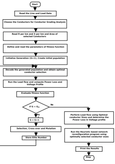
Branch currents of base network using Load flow program [15] are presented in Table. 1. Conductors are selected for optimization based on branch currents are given in Appendix. A2. To solve this conductor optimization, assume uniform conductor for base network. Optimal branch conductor selection has been performed with Genetic Algorithm (GA) approach as minimizing objective function given in equation (1). After obtaining optimal conductor sizes, load flow [15] is performed. Power loss and voltage profile are computed. The conductor optimization is explained in the proposed algorithm and flow chart as presented in Fig. 1. Selection of optimal conductor sizes is the first stage of this proposed method and a heuristic based reconfiguration [17] with obtained optimal conductor sizes is the second stage as shown in the flow chart.
PROPOSED ALGORITHM FOR NETWORK RECONDUCTORING
The proposed algorithm for reconductoring including projected load growth contains the following steps: 1. Read line and load data including branch lengths;
2. Choose type of conductors for branch conductor grading based on maximum load current of the network; 3. Read area and cost per km of chosen conductors for optimization;
4. Read parameters of fitness function;
5. Initialize population G=1 and create initial population;
6. Decode generated population, obtain conductor selection of each branch; 7. Run the proposed load flow method to compute power loss and voltage profile; 8. Evaluate fitness function;
9. If generation G< Gm(Gm is specified), go to next step else go to step 16;
10. Increment generation G=G+1;
11. Perform Genetic Algorithm operations such as selection, cross over and mutation; 12. Store elite number, go to step 6;
13. Store optimal branch conductors, power loss and Voltage profile of reconductoring with optimal selected conductors;
14. Compute Power loss and Voltage profile using heuristic based network reconfiguration with optimal graded conductor sizes;
15. Print the results; 16. Stop.
Table 1: BRANCH CURRENTS OF 33 BUS SYSTEM
Branch
Number Branch Current Before Grading After Grading Maximum Current carrying Capacity
1 364.139 Ferret Cat 390
2 323.8547 Ferret Cat 390
3 233.0174 Ferret Rabbit 228
4 221.169 Ferret Cat 390
5 216.4297 Ferret Cat 390
6 101.1058 Ferret Rabbit 228
7 82.1485 Ferret Cat 390
8 63.98104 Ferret Weasel 150
9 58.45182 Ferret Cat 390
10 52.92259 Ferret Rabbit 228
11 48.18325 Ferret Rabbit 228
12 42.65403 Ferret Rabbit 228
13 36.33491 Ferret Ferret 200
14 24.48657 Ferret Rabbit 228
15 19.74724 Ferret Rabbit 228
16 14.21801 Ferret Rabbit 228
17 8.688784 Ferret Cat 390
18 31.59558 Ferret Cat 390
19 23.69668 Ferret Cat 390
20 15.79779 Ferret Ferret 200
21 7.898894 Ferret Weasel 150
22 83.72828 Ferret Cat 390
23 75.82938 Ferret Cat 390
24 37.91469 Ferret Rabbit 228
25 112.9542 Ferret Cat 390
26 108.2148 Ferret Cat 390
27 103.4755 Ferret Cat 390
28 98.73618 Ferret Cat 390
29 87.67773 Ferret Cat 390
30 40.28436 Ferret Cat 390
31 26.06635 Ferret Cat 390
32 6.319115 Ferret Rabbit 228
Start
Read the Line and Load Data
Choose the Conductors for Conductor Grading Analysis
Read R per km and X per km and Area of selected Conductors
Define and read the parameters of fitness function
Initialize Generation (G=1), Create initial population
Decode the generated population and obtain optimal conductor selection
Run the Load flow and compute Power Loss and Voltage Profile
Evaluate fitness function
If G < Gm
G = G+1
Selection, Cross over and Mutation
Store Elite Number
Perform Load flow using Optimal conductor Sizes and determine the
Power Loss in Voltage profile
Run the Heuristic based network reconfiguration program using optimally selected conductor sizes
Print the Results
Stop
Ye s
Fig. 2: GA Optimization of 33 bus system
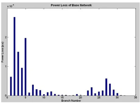
Fig. 3: Branch currents of base network
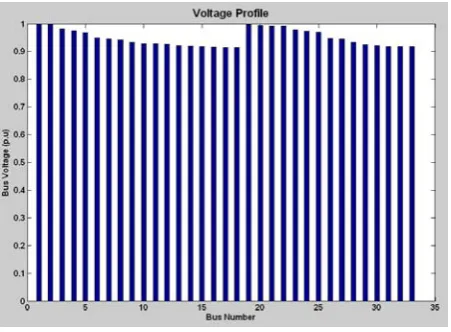
Fig. 4: Voltage profile of base network
0 20 40 60 80 100 120 140 160 180 200
2.9 3 3.1 3.2 3.3 3.4 3.5 3.6 3.7
3.8x 10
7
Population Size
Co
st
i
n
Ru
p
ees
Fig. 5: Branch power loss of base network
Fig. 2 shows the genetic optimization of conductors of a 33 bus system for a population of 200. Branch currents, bus voltages and branch power losses of bases network as shown in Fig. 3 – Fig. 5
b. Second Stage: Network Reconfiguration
In this method, a heuristic search is used [17] for determining the minimum loss configuration of the radial distribution system. For this algorithm, the resultant network of the first stage is taken as input. The proposed solution starts with initial configuration with all tie switches are in open position. The voltage differences across all tie switches and the two node voltages of each tie switch are computed using load flow analysis. Among all the tie switches, a switch with maximum voltage difference is selected first subject to the condition that the voltage difference is greater than the pre-specified value. The tie switch with the maximum voltage difference is closed and the sectionalize switches are opened in sequence starting from the minimum voltage node of the tie switch. The power loss due to each sectionalize switch is calculated and the procedure is terminated when the power Loss obtained due to previous sectionalizing is less than the current one. Based on the above procedure, the best switching combination of the loop is noted. This procedure is repeated to all the remaining tie switches. This procedure favors the solution with a fewer switching operations. Another advantage with the algorithm is that the number of load flow computations is less and subsequently the computational effort is significantly reduced.
Simulation Results:
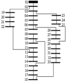
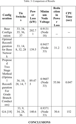
The proposed method has been tested on IEEE 33 radial distribution system [3] to demonstrate its effectiveness. This network has 33 buses, 32 branches and 5 tie lines as shown in Fig. 6. All the calculations for this method are carried out in the p.u. system with 12.66 kV and 100 MVA base. The convergence value ‘€’ is taken as 0.0001. The power losses and voltage profile were calculated and presented in Table. 3 .The results are determined in three configurations viz base network, optimal reconfiguration network and optimal reconfiguration with graded conductor sizes. Four conductors are taken to optimize the conductor sizes of this method. Line and Load data are presented in the Appendix. A1. The proposed algorithm is implemented in MAT lab. For this algorithm, Dual core 1 GB RAM, 1.66 GHz system was used.
and minimum voltage of the graded network are 115.791 kW and 0.9428 (at Node 33) p.u respectively. In the second stage of proposed method the optimal conductor sizes are used in the base network and implemented heuristic method to reconfigure the system the power loss and minimum voltage obtain from final configuration are 89.473 kW and 0.9607 p.u (at Node 33). Optimal switch configuration of the proposed method are 36, 10, 28, 14 and 7 as shown in Fig. 8
Fig. 6: IEEE 33 Bus radial distribution system
Fig. 7: Optimal final configuration after all switching operations
Simulation Results:
Table. 2: Comparison of voltages
B U S N U M B E R Node voltag e in p.u. (Befor e gradin g) Node voltag e in p.u. (After gradi ng) Node volta ge in p.u. (Two Stage Prop osed Meth od) B U S N U M B E R Node voltag e in p.u. (Befo re gradi ng) Node volta ge in p.u. (Afte r gradi ng) Node voltag e in p.u. (Two Stage Propo sed Metho d) 1 1.000
0 1.000 1.0000 18 0.8983
0.942 8 0.9638 2 0.997 0 0.998 2 0.998 2 19 0.996 5 0.998 0 0.9973 3 0.982
9 0.9898 0.9920 20 0.9929 0.9961 0.9891 4 0.975
5 0.9835 0.9905 21 0.9922 0.9955 0.9856 5 0.968
1 0.9791 0.9896 22 0.9916 0.9949 0.9828 6 0.949 7 0.969 8 0.987 9 23 0.979 4 0.987 9 0.9877 7 0.946
2 0.9685 0.9877 24 0.9727 0.9843 0.9796 8 0.941
3 0.9654 0.9750 25 0.9694 0.9817 0.9708 9 0.935
1 0.9581 0.9711 26 0.9477 0.9686 0.9878 10 0.929 2 0.954 9 0.970 8 27 0.945 2 0.967 1 0.9876 11 0.928
4 0.9542 0.9767 28 0.9337 0.9614 0.9873 12 0.926
9 0.9528 0.9768 29 0.9255 0.9574 0.9655 13 0.920
8 0.9482 0.9749 30 0.9220 0.9552 0.9633 14 0.918 5 0.946 5 0.974 3 31 0.917 8 0.953 1 0.9613 15 0.917
1 0.9454 0.9664 32 0.9169 0.9527 0.9609 16 0.915
7 0.9444 0.9564 33 0.9166 0.9608 0.9608 17 0.913
Voltage Profile Base Netwrok Optimal Graded Netwrok Two Stage Proposed Method
4 8 12 16 20 24 28 32 36
0.88 0.9 0.91 0.92 0.93 0.94 0.95 0.96 0.97 0.98 0.99 1 V ol tage (p .u .) Node Number
Fig. 9: Voltage Comparison
Table. 3: Comparison of Results
Config uration Tie Switche s Pow er Loss (kW) Minim um Node Voltage Redu ction in Powe r Loss CPU Time (sec) Base Configu ration 33, 34, 35, 36, 37 202.7 1 0.9131 (Node
18) -- -- Optimal Reconfi guration for Base Networ k 33, 14,
8, 32, 28 139.5
0.9437 (Node 33) 31.2 5.3 Propose d Two Stage Method (Optima l Reconfi guration For Grade Branch Conduct ors) 36, 10,
28, 14, 7 89.473
0.9607 (Node
33) 55.86 0.047
GA [18] 34, 28, 33, 9,
36 140.6
0.9371 (Node
33) 30.6 152
CONCLUSIONS
AKNOWLEDGEMENTS
The authors are thankful to EPDCL Company, Andhra Pradesh, India for providing data used in this work.
APPENDIX A
Table. A1: Line and Load data of 33 Bus System:
B R A N C H N U M B E R S E N D I N G E N D B U S R E C E I V I N G E N D B U S
Base Case Optimal Case End Bus Loads
R (Ω) X (Ω) R (Ω) X (Ω)
PL (kw) QL (kw)
1 1 2 0.9922 0.047 0.0526 0.0216 100 60
2 2 3 0.4930 0.2511 0.2769 0.1136 90 40
3 3 4 0.3660 0.1844 0.2049 0.08408 120 80
4 4 5 0.3811 0.1941 0.2135 0.0876 60 30
5 5 6 0.8190 0.7070 0.4588 0.18824 60 20
6 6 7 0.1872 0.6188 0.1047 0.04296 200 100
7 7 8 0.7114 0.2351 0.9594 0.3936 200 100
8 8 9 1.0300 0.74 0.5772 0.2368 60 20
9 9 10 1.0440 0.74 0.5830 0.2392 60 20
10 10 11 0.1966 0.065 0.1689 0.04689 45 30
11 11 12 0.3744 0.1238 0.4063 0.09245 60 35
12 12 13 1.4680 1.155 0.8209 0.3368 60 35
13 13 14 0.5416 0.7129 0.312 0.128 120 80
14 14 15 0.5910 0.526 0.8908 0.153 60 10
15 15 16 0.7463 0.545 0.8106 0.18443 60 20
16 16 17 1.2890 1.721 0.7222 0.29632 60 20
17 17 18 0.7320 0.574 0.4095 0.168 90 40
18 2 19 0.1640 0.1565 0.1408 0.03911 90 40
19 19 20 1.5042 1.3554 0.8424 0.3456 90 40
20 20 21 0.4095 0.4784 0.2293 0.09408 90 40
21 21 22 0.7089 0.9373 1.0674 0.18333 90 40
22 3 23 0.4512 0.3083 0.2535 0.104 90 40
23 23 24 0.8980 0.7091 0.5031 0.2064 420 200
24 24 25 0.8960 0.7011 0.5011 0.2056 420 200
25 6 26 0.2030 0.1034 0.113 0.04664 60 25
26 26 27 0.2842 0.1447 0.1591 0.06528 60 25
27 27 28 1.059 0.9337 0.5933 0.24344 60 20
28 28 29 0.8042 0.7006 0.4504 0.1848 120 70
29 29 30 0.5075 0.2585 0.2847 0.1168 200 600
30 30 31 0.9744 0.963 0.546 0.224 150 70
31 31 32 0.3105 0.3619 0.1739 0.07138 210 100
32 32 33 0.341 0.5302 0.1910 0.07838 60 40
33* 21 8 2 2 2 2 Tie Line
34* 9 15 2 2 2 2 Tie Line
35* 12 22 2 2 2 2 Tie Line
36* 18 33 0.5 0.5 0.5 0.5 Tie Line
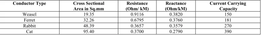
Table. A2: Conductor Data:
Conductor Type Cross Sectional Area in Sq.mm
Resistance (Ohm/ kM)
Reactance (Ohm/kM)
Current Carrying Capacity
Weasel 19.35 0.9116 0.3820 150
Ferret 32.26 0.6795 0.3760 181
Rabbit 48.39 0.3657 0.3579 270
Cat 95.40 0.3700 0.2790 390
REFERENCES
[1] Merlin, H. Back, “Search for a minimal-loss operating spanning tree configuration in an urban power distribution system” proceedings
of Power system Computation Conference(PSCC), Cambridge, UK,1975, pp 1-18.
[2] D. Shirmohammadi and H. W. Hong,”Reconfiguration of electrical distribution networks for resistive line loss reduction,”IEEE Trans.
On Power Delivery, Vol. 4, No. 2, April 1989, pp. 1492-1498.
[3] M. E. Baran and F. F. Wu,”Network reconfiguration in distribution systems for loss reduction and load balancing,” IEEE Trans. On
Power Delivery, Vol. 4, No. 2, April 1989 pp. 1401-1407.
[4] Civlnar, S.; Grainger, J. J.; Yin, H; Lee, S. S. H., Distribution feeder reconfiguration for loss reduction, IEEE Trans. On Power
Delivery, Vol. 3, 1988.
[5] T. Thakur and Jaswanti, ”Study and characterization of power distribution network reconfiguration”, Proc. of IEEE, 2006.
[6] Ponnavaiko M and Rao K.S.P, "Optimal Distribution System planning", IEEE Trans. on PAS, June 1981, pp. 2969-2977.
[7] Tram H.N and Wall D.L, "Optimal Conductor selection in planning radial distribution systems", IEEE Trans. On Power Systems,
Vol.3, No. 1, pp. 200-206, Feb 1988.
[8] Wang et al. “A practical approach to the conductor size selection in planning radial distribution system”, IEEE Trans. on Power
Delivery, Vol. 15, No. 1, Jan 2000, pp. 350-353.
[9] D. Das, H.S. Nagi, D.P. Kothari, “Novel method for solving radial distribution networks”, IEE Proc.gen. Trans. Distrib, Vol. 141, No.
4, July 1994, pp. 291-298.
[10] Smarajit Ghosh, U. S. Chhatwal, “Enhancement of loadingof Radial Distribution Networks Using Optimal Conductor Size”,
International Journal of computer and Electrical Engineering, Vol. 1, No. 2, June 2009, pp. 126-134.
[11] R. Ranjan et al, “Optimal conductor selection of radial distribution feeders using Evolutionary programming”, proc. IEEE, 2003.
[12] Sivanagaraju et al. “Optimal Conductor Selection for Radial Distribution,” Elsevier, Electric Power System Research, Vol. 63, 2002,
pp. 95-103.
[13] Franklin Mendoza et al. ” Optimal Conductor Size Selection in Radial Power Distribution Systems Using Evolutionary Strategies”,
IEEE PES Transmission and Distribution Conference and Exposition Latin America, Venezuela, 2006.
[14] Ramesh et al., “Minimization of power loss in distribution networks by different techniques”, International journal electrical power
and energy systems engineering, Vol. 2, No. 1, 2009.
[15] G. R. Regulavalasa, S.R. Annapragada, V.L.N. Sadhu, H.R. Bhaganagarapu, “A Novel method for optimal conductor selection of
distribution networks using Genetic Algorithm”, International Review of Modeling and Simulation(IREMOS), Vol. 1, N. 1, Oct. 2008, pp. 178-181.
[16] Marvasti et al., “Combination of Optimal Conductor Selection and Capacitor Placement in Radial Distribution Systems for Maximum
Loss Reduction”, IEEE international conference on Industrial Technology (ICIT), 2009.
[17] Srinivasa Rao, R.; Narasimham, SVL, A Novel heuristic approach for network reconfiguration in large scale distribution systems,
International Journal of applied Science, Engineering and Technology, Vol. 5, No. 1, Jan. 2009, pp 15-21.
[18] Y.Y. Hong and S.Y. Ho, “Determination of network configuration considering multi-objective in distribution systems using genetic
algorithms, “IEEE Trans, Power Syst., vol.20, no.2, May 2005, pp. 1062-1-69.
BIOGRAPHIES
R. Gowrisankara Rao, Graduated from Andhra University, Visakhapatnam, AP, INDIA and obtained M. Tech. in Power Systems from JNTU, Kakinada, INDIA. Presently he is Head of the department, Electrical and Electronics Engineering, MVGR College of Engg., Vizianagaram, INDIA. His area of interest is Electrical Distribution System.
Dr.S.V.L.Narasimham is Professor of Computer Science and Engg., Jawaharlal Nehru Technological University, Hyderabad, India. He has published more than 20 papers in National and International Journals. His areas of interests include real time power system operation and control, ANN, Fuzzy logic and Genetic Algorithm applications to power Systems.