VISCOELASTIC MODELING OF
GROUND RESPONSE TO STRONG
SURFACE WAVES
RAJNEESH KAKAR
Principal
DIPS Polytechnic College, Hoshiarpur-146001, India E-mail: [email protected]
MONIKA RANI
Research Scholar
Punjab Technical University, Jalandhar,144601, India
K. C. GUPTA
Supervisor
Punjab Technical University, Jalandhar,144601, India
Abstract:
Since soil dynamic behaviour is nonlinear in nature therefore a nonlinear viscoelastic model for isotropic materials is proposed in this study. This model is a combination of inelasticity and nonlinear damping. In this model, the shear modulus is taken as a function of the excitation level. The viscosity is assumed to vary non-linearly. The validity of this model is checked for low amplitude ground motion response towards strong seismic waves. This method is imposed into a one dimensional finite element approach for a dry soil. The validation of this model is studied for cyclical loading. This model is based on the principle of nonlinear elasticity and nonlinear viscoelasticity which investigate the ground response to strong surface waves excitation. Finally, finite element method is introduced for numerical calculations.
Mathematics Subject Classification: 74S05; 74D10; 74J15; 74J30.
Keywords: Nonlinear Wave Propagation; Surface Waves; Finite Element Method. 1 Introduction
The dynamic response of unconsolidated soils cannot generally be investigated directly. Therefore, the analysis of dynamic soils is studied with some special experimental methods Semblat [1]. With the help of wave propagation the dynamic and vibratory excitations on soil can be analyzed. Bard and Bouchon [2], Paoluci [3] and Semblat et al. [4] investigated resonance at the scale of the whole basin. Also, Bard and Thomas [5], Bozzano et al. [6] and Kawase [7] studied generation of surface waves at the egde of basin. Vucetic [8] discussed normalized behaviour of clay under irregular cyclic loading. Jankowski [9] discussed the linear viscoelastic model and the nonlinear viscoelastic model. Anagnostopoulos [10] studied the linear viscoelastic model of collision to simulate structural pounding. Jankowski et al. [11] studied the pounding of superstructure segments in bridges with the help of linear viscoelastic model. Muthukumar and DesRoches [12] made a comparison study using two single degree of freedom (SDOF) systems for capturing pounding. Westermo [17] suggested linking buildings with beams which can transmit the forces between them eliminating dynamic contacts . Bonilla et al.[14] discussed nonlinear nature of soils at the geotechnical scale. Recently, Kaur et al. [21] discussed nonlinear dynamic loading of viscoelastic solids.
2 Formulation of the model
2.1 Basic relations for 3D linear viscoelasticity
2.1.1 General formulation
We consider 3D formulation of the viscoelastic model by using the relation (Bourbié et al.) [22]
ij
s
ijp
ij
(1)where ij is Cauchy stress tensor, sij is stress tensor, ij Kronecker unit tensor and p is volumetric tension respectively.
For an isotropic material, volumetric tension can be written as
p=K ekk (2)
where K is bulk modulus and ekk is volumetric strain respectively.
For linear viscoelasticity, the relation between the Fourier transform components of stress tensor s and shear strain tensor e is
sij ()=2M()eij() (3)
M() is viscoelastic modulus parameter, which is complex and frequency-dependent. The specific attenuation
Q-1 is given by (Semblat (2009) [23]
1
Im(
( )
2
( )
Re(
( )
M
Q
M
(4)where is the damping ratio.
2.1.2 Nearly constant attenuation models
In fig. 1, the nearly constant attenuation model is shown (Emmerich and Korn) [23]. It is generalized Maxwell body having viscosities
a
l.
M
/
l and elastic modulia
l.
M
. This type of models is expressed in term of the quality factor Q. In such types of models Q is kept constantfor a given strain level.R t( )
MU
MR
M
t=0 time
a Ml
a M/l l
M
Fig. 1. Generalized Maxwell model and its rheological cell
In this model,
R t
( )
is relaxation function ,M
Uis the un-relaxed modulus andM
Rrepresents the relaxed modulus. The frequency dependent complex modulus for generalized Maxwell model is( ,0) ( )
( ,0)
1 ( ) 1
( )
1
1
(
)
n n
l l
U l
l l l
y
M
M
y
i
(5)The variables ( ,0)l
y
are characterize the viscoelastic model and can be calculated for obtain a nearly constant attenuation in a given frequency range by using Emmerich and Korn’s method. We consider the viscoelastic model depicted in Fig. 1.To estimate the a(l) coefficients, a normalization condition is introduced) ( )
0 ,
( l
R
l
a
M
M
y
(6)Using Eq. (4) and (5), the quality factor has the following expression: 2
( ) ( )
1
( ,0) 2 ( ,0) 2
1 ( ) 1 ( )
/
( /
)
( )
1
1 ( /
)
1 ( /
)
n n
l l
l l
l l l l
Q
y
y
Where,
(l) represents the frequency of single rheological cellThe relation for the linear viscoelastic model can be written as
n
l l ij
U
ij
t
M
e
t
t
s
1 ) (
(
)
)
(
2
)
(
(8)and
)
(
1
)
(
)
(
1 ) 0 , ( ) 0 , ( ) ( )
( ) ( )
(
e
t
y
y
t
t
n ijl l l l l
l l
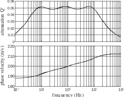
(9)where (l)(t) are relaxation parameters lth-cell (Fig. 1). Fig. 2 shows the attenuation curve (2=Q-1) and the phase velocity (Vph), as functions of frequency. The attenuation is nearly constant for 0.05, in the frequency range of 0.1-10Hz. The target phase velocity, |Vph|=200m/s, is chosen at a frequency of 1Hz.
0 0.01 0. 02 0. 03 0. 04 0. 05 0. 06
180 190 200 210 220
pha
se
ve
loc
it
y
(m
/s
)
a
tte
nu
atio
n
Q
-1
f req ue ncy (Hz )
10-2 10-1 100 101 102
Fig. 2. ( Nearly Constant Quality factor Q20)
2.2 3D nonlinear viscoelastic model
2.2.1 Formulation of the extended nearly constant attenuation model
We have introduced a dissipation function and an elastic potential function. Both these functions depend on the magnitude of the second invariant of the strain tensor. These functions explain the dynamic nature of the soil i.e. shear modulus and damping variations with the excitation level. The model is in agreement to time domain formulations. Further, we put a dependence on the excitation level. This dependence can be controlled by varying second order invariant of the strain tensor.
In order to study the non linear behaviour of soils for any 3D stress-strain path, Eq. (8) can be written as
n
l
l l ij
U
ij
t
M
J
e
t
t
y
J
s
1
2 ) ( ) (
2
)
(
)
(
,
(
))
(
2
)
(
(10)J2 (the second invariant of the strain tensor) is
3
2 ' 1 ' 2 2
I
I
J
(11)where,
)
(
'
1
trace
I
(12)and
)
(
2
1
2'
2
trace
I
(13)Further, the shear modulus is
1
(
)
)
(
J
2M
,0J
2Shear modulus is assumed to change during the stress-strain path. where,
2 1 2 2 1 2 2
1
)
(
J
J
J
(15)MU,0 represents the un-relaxed modulus. It is responsible for the instantaneous response of the soil at small strains. is a parameter represents the nonlinear behaviour of larger strains.
We now introduced the octahedral strain
oct as2 1 2
2
J
oct
(16)It gives to
1
(
)
)
(
oct U,0 octU
M
M
(17)where,
2
/
1
2
/
)
(
oct oct
oct
(18)From the above equation, octahedral strain
oct depends on the variables y(l) and (l). In the case of 3Dloadings, an extension of related as
[25]
(Bonnet and Heitz) [25])
(
)
(
)
(
oct
0
max
0
oct
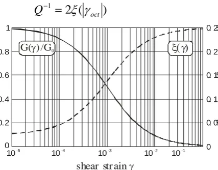
(19)where 0 is the energy dissipated in the small grains andmaxis the energy dissipated in the larger strain ranges respectively. In Fig. 3, shear modulus reduction (solid) and damping increase (dashed) with increasing shear strain is displayed for typical MU()=G() and ()
Therefore, the damping ratio and the attenuation Q-1 are now related by
)
(
2
1
oct
Q
(20)10-5
10-4
10-3
10-2
10-1
0 0.2 0.4 0.6 0.8 1
shear str ain
0 0. 05 0. 1 0. 15 0. 2 0. 25
G( ) /G 0
Fig. 3. Typical nonlinear dynamic properties of soils
2.2.2 Features of the extended nearly constant attenuation model
The solution of Eq. (10) is found in the limit of low excitation levels. Hence, for low octahedral strains, we can assume
0 1 0
2
Q
(21)and
0 0 ,
)
0
(
M
G
M
U
oct
U
(22)only the variables y(l,0) change to account for the variation of the damping with strain in Eq. (7). Hence, we have introduced a strain variation of the variables y(l) with strain in the following form:
) 0 , ( )
(l
(
oct)
c
(
oct)
y
ly
(23)Using Eqs. (4), (16) and (18) in Eqs. (5) and (24), we get
n l l oct n l l l l oct oct U octy
c
i
y
c
M
M
1 ) 0 , ( 1 ) ( ) ( ) 0 , ()
(
1
)
/(
)
(
1
)
(
)
,
(
n l l l l octoct
c
y
Q
1 2 ) ( ) ( ) 0 , ( 1/
1
/
)
(
)
,
(
(25) (26) where,
)
(
1
)
(
)
,
(
)
(
0 0 max 0 1 0 1 oct oct oct octQ
Q
c
(27)Eq. (9) can be written in the more general form as
)
(
)
(
1
)
(
)
(
)
(
1 ) 0 , ( ) 0 , ( ) ( ) ( ) ( )(
e
t
y
c
y
c
t
t
n ijl l oct l oct l l l l
(28)Eq. (10) can be solved in the time domain with the help of latter expression and Eq. (17). 2.3 Special case
For a shear wave propagating in 1D, |oct| = 2||, where is the shear strain. Therefore, Eq. (17) can be written in the form
1
)
(
)
(
G
G
0M
U (29)In this case, Eq. (29) represents a hyperbolic law for the reduction of the shear modulus which is in complete agreement with the results of Hardin and Drnevich [26]. As a result, we get the following equation for the function c(|oct|)
1
1
)
(
0 0 maxc
(30)where max and 0are two experimental values. At every time, the values associated to the functions (l)(t) are obtained by solving the following equations:
)
(
)
(
1
)
(
)
(
)
(
1 ) 0 , ( ) 0 , ( ) ( ) ( ) ( )(
e
t
y
c
y
c
t
t
n l l l l l l l
(31)Finally, Eq. (10) is used for the considered 1D case:
n l l lt
y
t
e
G
t
s
1 ) ( ) (0
(
)
(
,
(
))
1
2
)
(
(32)3 Cyclic loadings of the model for validation
0
0
0
0 -1000
-500 0 500 1000
(Pa
)
-2.104
0 2.104
- 10-5
-5.10-4
-10-4
-10-3
10-5
5.10-4
10-4
10- 3
(Pa
)
- 4.104
- 2.104
0 2.104
4.104
-5000 0 5000
r=0.99 r=0. 91
r=0.77 r=0.5
NM 1st loading
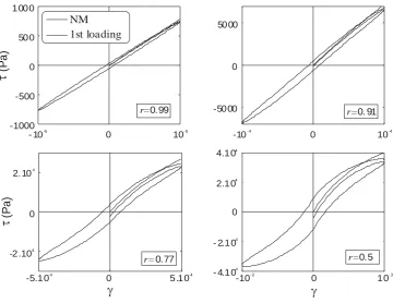
Fig. 4. Stress-strain curves for cyclic loadings
The various parameters for sinusoidal cyclic loadings are chosen as =1000 and G0=80MPa. The relaxation parameters can be computed from Eqs (30) and (31) by using 0=0.025 and max=0.25 (the asymptotic damping values). Fig. 4 is plotted at 10Hz and stress-strain loops are obtained for max=10-5, 10-4, 5.10-4 and 10-3. For
each case, G is computed and normalized by G0 ( 0
G
r
G
is given in each curve). The solid line in the curve isfor nonlinear extended nearly constant attenuation model and dashed line is for 1st loading curve. From these curves, we can solve secant shear modulus G as a function of maximum shear strain. The area under each loop gives the dissipation energy. The damping ratio can easily be derived from this energy ratio.
0
0
0
0 -1000
-500 0 500 1000
(Pa
)
-2.104
0 2.104
- 10-5
-5.10-4
-10-4
-10-3
10-5
5.10-4
10-4
10- 3
(Pa
)
- 4.104
- 2.104
0 2.104
4.104
-5000 0 5000
r=0.99 r=0. 91
r=0.77 r=0.5
NM 1st loading
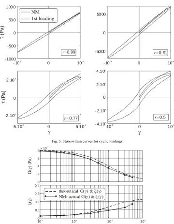
Fig. 5. Stress-strain curves for cyclic loadings
0 0 .1 0.2 0.3 0.4
0
2 4 6
8x 10
7
10-5 10-4 10-3 10-2
theo retical G( ) & ( ) NM: actu al G( ) & ( )
G(
) (
P
a
)
()
Fig. 6. Comparison of the shear modulus and damping values (%) of the extended nearly constant attenuation model under cyclic loadings
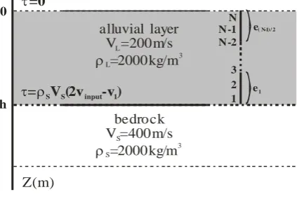
Numerical implementation (FEM)
0
h
alluvial layer V =200m/s
=2000kg/m
L
L
3
N N-1 N-2
3 2 1
e( N-1)/ 2
e1
=0
= SV (2vS input-v )1
Z(m)
bedrock V =400m/s
=2000kg/m
S
S
3
Fig. 7. 1D soil layer
We have divided the domain is into (N-1)/2 linear quadratic finite elements. Each finite element consists of the
N nodes having 1 degree of freedom. The equation of motion for each time step (n+1)t is
max 1
n ) ( )
( ) ( )
(
1 1
1 1
1
,
1
;
)
u
(
)
(
)
(
)]
(
[
]
[
]
[
l
l
H
t
t
F
u
u
K
v
C
a
M
l l
l l
n n
n n
n
(33)where [M], [C] and [K(un+1)] represent the mass, the radiation condition at the bedrock/layer interface (elastic substratum), and the stiffness matrix respectively. {an+1}, {vn+1} and {un+1} are the acceleration, velocity and displacement vector respectively, while {Fn+1} is the vector of external forces at the interface. (l) and (l) are the relaxation parameters and central frequencies of the rheological cells (resp.), H(l)(un+1) corresponds to the right hand-side term in Eq. (31) and lmax is the total number of cells included in the model (lmax=3 herein).
4 Modeling wave propagation in the nonlinear range 4.1 Nonlinear layered model
We have performed modeling wave propagation in the nonlinear range for two types of simulations
Linear attenuating model
Nonlinear extended nearly constant attenuation modelFor the first one (0=max=2.5% and ), the mechanical and dissipative properties of the material do not depend on the excitation level while, in the second case (0=2.5%, max=25% and ), both elastic and dissipative properties are function of the induced strain as shown in Figs 3 and 5. For both models, we performed simulations for a 15 m deep soil layer over elastic bedrock, with a velocity contrast of 2 and an absorbing condition at the bottom of the layer (Fig. 6). The excitations considered hereafter thus correspond to the incident wavefield at the top of the bedrock.
4.2 Sinusoidal incident wave
We have considered sinusoidal incident wavefield for 2 seconds, which is given as
0 0
)
sin
sin(
)
(
t
t
t
a
with
0
2
f
0 andf
0
3
Hz
(34)Fig. 8 is plotted for accelerations (left) and corresponding Fourier spectra (right) at the top of the soil layer, for 2 values of the maximum input acceleration on bedrock 0.5 (top) and 0.75 m/s2 (bottom): linear simulations are represented by dotted lines and nonlinear simulations with solid lines. The nonlinear time histories involve propagation time delays when compared to the linear ones, as it can be easily observed by comparing the peaks arrival times for both models in Fig. 7. In the latter case, the Fourier spectra of the nonlinear signals indicate:
1) a significant decrease of the spectral amplitude, with increasing excitation level, for the main frequency components of the input signal;
2) the generation of higher frequency peaks which are not contained in the input signal (around 3 and 5 times the predominant excitation frequency). Such higher frequency components are larger for stronger excitations (bottom) ;
-1.5 -1 -0.5 0 0.5 1 1.5
0 0.5 1 1.5 2 2.5 3
-1.5 -1 -0.5 0 0.5 1 1.5
0 0.1 0.2 0.3 0.4
0 5 10 15
0 0.1 0.2 0.3 0.4
NM: LM:
=1000
0=2.5%
0=2.5%
ma x=25%
time (s )
ac
cel
er
at
io
n
(
m
/s
)
2
FF
T
(
m
/s
)
FF
T
(
m
/s
)
ac
c
el
er
at
io
n
(
m
/s
)
2
frequency (Hz)
Fig. 9. Accelerations (left) and corresponding Fourier spectra (right) at the top of the soil layer
-1 -0.5 0 0.5
1x 1 0 -3
(t
)
0 1 2 3
-1 -0.5 0 0.5
1x 1 0 -3
time (s)
(t
)
-5 0 5
x 104
(
) (
P
a
)
-1 -0.5 0 0.5 1 x 10⁻³ -5
0 5
x 104
(
) (P
a
)
LM NM 1s t loadi ng
Fig. 10. Shear strains (left) and stress-strain loops (right) at the middle of the soil layer,
The shear strain at the centre of the layer is also plotted in Fig. 8 (left) for both excitation levels. Similar time delays are observed in the time-histories. From the stress-strain paths (Fig. 8, right), the reduction of the shear modulus and the energy dissipation are found to be larger for peaks of increasing amplitudes. The largest effect is obtained for the strongest excitation (Fig. 8, bottom right). Fig. 8 represents two values of the maximum input acceleration on bedrock 0.5 (top) and 0.75 m/s2 (bottom): linear (dotted) and nonlinear (solid) simulations. 5 Conclusions
A 3D nonlinear viscoelastic model is proposed to approximate the hysteretic behaviour of unconsolidated layer deposits undergoing surface wave excitation. Such nonlinear features as the reduction of shear modulus and the increase of damping are controlled by the variations of the 2nd invariant of the strain tensor during multidimensional loading. In the case of a unidirectional shear loading, nonlinearity is controlled by only one shear strain component: nonlinear elasticity by a hyperbolic law and viscosity by a nearly constant attenuation model with nonlinear features (nearly frequency constant but strain amplitude dependent).
Acknowledgements
The authors would like to thank Dr. Shikha Kakar for fruitful discussions. Nomenclature:
{a} = acceleration vector (FEM)
[C] = damping matrix (FEM)
e = shear deviatoric strain tensor
eij() = Fourier transforms of the components of the deviatoric strain
ekk = volumetric strain
oct = octahedral strain
ij = Kronecker unit tensor components
M = difference between the relaxed and un-relaxed moduli l(t) = relaxation functions
0 = minimum damping at low strains max = maximum damping at large strains ij = components of the Cauchy stress tensor = function characterizing the modulus reduction
= circular frequency
f = frequency
{F} = external force vector (FEM)
Q = quality factor
Q-1 = specific attenuation
s = shear deviatoric stress tensor
sij = components of the deviatoric stress tensor
sij() = Fourier transforms of the components of the deviatoric stress
{u} = displacement vector (FEM)
{v} = velocity vector (FEM)
y(l,0) = relaxation parameters of the viscoelastic cells for low excitation levels = scalar parameter characterizing the modulus reduction
G0 = (unrelaxed) shear modulus at low strains
I’1 = first invariant of the strain tensor
I’2 = second invariant of the strain tensor
J2 = second invariant of the deviatoric strain tensor
K = bulk modulus
[K] = tangent stiffness matrix (FEM)
M() = complex viscoelastic modulus
[M] = mass matrix (FEM)
MR = relaxed modulus
MU = unrelaxed modulus
MU,0 = unrelaxed modulus at low strains
p = volumetric tension
References
[1] Semblat, J.F. (1995): Soils under dynamic and transient loadings: dynamic response on S.H.P.B, wave propagation in centrifuge
medium, Rapport Etudes et Recherches des L.P.C, Laboratoire Central des Ponts et Chaussées. Paris, pp 206.
[2] Bard, P.Y.; Bouchon, M. (1985): The two dimensional resonance of sediment filled valleys. Bull. Seism. Soc. Am.,75, pp 519-541.
[3] Paolucci, R. (1999): Shear resonance frequencies of alluvial valleys by Rayleigh’s method. Earthquake Spectra, 15, pp 503-521.
[4] Semblat, J.F.; Paolucci R.;Duval, A.M. (2003): Simplified vibratory characterization of alluvial basins. C.R. Geoscience, 335, pp
365-370.
[5] Bard, P.Y.; Riepl-Thomas, J. (2000): Wave propagation in complex geological structures and their effects on strong ground motion.
Wave motion in earthquake eng., Kausel and Manolis eds, WIT Press, Southampton, Boston, pp 37-95.
[6] Bozzano, F.; Lenti, L.; Martino, S.; Paciello, A.; Scarascia Mugnozza, G. (2008): Self-excitation process due to local seismic
amplification responsible for the reactivation of the Salcito landslide (Italy). J. Geophys. Res., pp 113, B10312, doi:10.1029/2007JB005309.
[7] Kawase, H. (2003): Site effects on strong ground motions, International Handbook of Earthquake and Engineering Seismology, Part
B, W.H.K. Lee and H. Kanamori (eds.). Academic Press, London, pp 1013-1030.
[8] Vucetic, M. (1990): Normalized behaviour of clay under irregular cyclic loading. Can. Geotech. J., 27, pp 29-46.
[9] Jankowski, R. (2005): Nonlinear Viscoelastic Modelling of Earthquake-Induced Structural Pounding. Earthquake Engineering and
Structural Dynamics 34(6), pp 595-611.
[10] Anagnostopoulos, S.A. (1988): Pounding of Buildings in Series during Earthquakes. Earthquake Engineering And Structural
[11] Jankowski, R.; Wilde, K.; Fujino, Y. (1998): Pounding of Superstructure Segments In Isolated Elevated Bridge During Earthquakes. Earthquake Engineering and Structural Dynamics 27, pp 487-502.
[12] Muthukumar, S.; Desroches, R. (2006): A Hertz Contact Model with Nonlinear Damping for Pounding Simulation. Earthquake
Engineering and Structural Dynamics 35, pp 811-828. Semblat, J.F.; Duval, A.M.; Dangla, P. (2000): Numerical analysis of seismic wave amplification in Nice (France) and comparisons with experiments, Soil Dynamics and Earthquake Eng.,19(5), pp 347-362.
[13] Sugito, M. (1995): Frequency–dependent equivalent strain for equi-linearized technique. Proc. First International Conference on
Earthquake Geotechnical Engineering; 1(A), pp 655-660.
[14] Bonilla, L.F.; Li, P.C.; Nielsen, S. (2006): 1D and 2D linear and non linear site response in the Grenoble area. Proc. 3rd Int. Symp. on
the Effects of Surface Geology on Seismic Motion, University of Grenoble, LCPC, France.
[15] Christensen R.M. (1971). Theory of Viscoelasticity. An Introduction, Academic Press, New York.
[16] Malvern, L.E. (1969): Introduction to the Mechanics of a Continuous Medium, Prentice Hall, New Jersey.
[17] Westermo, Bd. (1989): The Dynamics of Interstructural Connection to Prevent Pounding. Earthquake Engineering Andstructural
Dynamics; 18, pp 687–699.
[18] Lakes, R.S. (1998). Viscoelastic solids. CRC Press, New York,
[19] Findley, W.N.; Lai, J.S.; Onaran, K. (1976): Creep and relaxation of nonlinear viscoelastic materials. Dover, New York.
[20] Oden, JT. (1972). Finite Elements for Nonlinear Continua. McGraw Hill.
[21] Kaur, K.; Kakar, R.; Gupta, K.C. (2012): A dynamic non-linear viscoelastic model. International Journal of Engineering Science and
Technology, 4 (12), pp 4780-4787.
[22] Bourbié, T. ; Coussy, O. ; Zinzsner, B. (1987) : Acoustics of porous media, Technip, Paris, France.
[23] Semblat, J.F.; Pecker, (2009): A. Waves and Vibrations in Soils: Earthquakes. Traffic, Shocks, Construction Works, IUSS Press,
Pavia, Italy, pp 500.
[24] Emmerich, H.; Korn, M. (1987): Incorporation of attenuation into time-domain computations of seismic wave fields. Geophysics,
52(9), pp 1252-1264.
[25] Bonnet, G.; Heitz, J.F. (1994): Nonlinear seismic response of a soft layer. Proc. 10th European Conf. on Earthquake Engineering,
Vienna, Balkema, pp 361-364.
[26] Hardin, B.O.; Drnevich, (1972): V.P. Shear modulus and damping in soils: Design equations and curves. Journal of Soil Mechanics