1.Introduction In recent years, singular integral equations arise in many problems of

The product Nyström method for solving nonlinear Volterra

integral equation with weakly kernel

F. A. Hendi *, Sh. A. Al-Hazmi**

*Department of Mathematics, Faculty of Science , King Abdul-Aziz University ,Jeddah ,Saudi-Arabia, E- mail: falhendi @kau.edu.sa

**Department of Mathematics, Girls Collage of Education , Umm Al -Qura University , Makkah, Saudi Arabia, E- mail: [email protected]

Abstract:::: In this work, the existence and uniqueness of the solution of the nonlinear Volterra integral equation with weakly kernels are discussed. Also, the product Nyström method is considered, to obtain a nonlinear system of algebraic equations.. In the later, we discuss numerically some examples, when the kernel takes a logarithmic and Carleman forms. Also the estimate error in each case, is calculated.

Key words: Singular nonlinear Volterra integral equation (SNVIE), Product Nyström method, Nonlinear algebraic system (NAS), Weakly singular kernel.

AMS : 45 B 05- 45 G 10 -65 R

1.Introduction

In recent years, singular integral equations arise in many problems of mathematical physics, such as the theory of elasticity, viscoelasticity, hydrodynamics. Also, many problems of fracture mechanics, aerodynamics, the theory of porous filtering, antenna problems in electromagnetic theory, viscodynamics fluids, contact problems in the theory of

elasticity, mixed boundary problems in mathematical physics, biology, chemistry and engineering and others can be formulated as integral equations of the first, second and third

kind, see Hendi and AL-Hazmi [1], Hochstadt [2], Kanwal [3], and Schiavone et.al [4].

The solutions of these problems can be obtained analytically, using the theory developed by Muskhelishvili [5,6]. At the same time the scene of numerical methods takes an important place in solving integral equations. Many methods are used to obtain the solution of the NIE, Abdalkhani [7] obtained a numerical solution of the NVIE of the second kind when the kernel takes Abel's function form. Guoqiang et. al [8], obtained numerically the solution of two-dimensional of the NVIE by collocation and iterated collocation methods.

In [9], Brunner et. al, introduced a class of methods depending on some parameters to obtain numerically the solution of Able's integral equation of the second kind. In [10] Kauthen applied a linear multistep method to obtain numerically a SVIE. In [11] Kibas and Saigo used an asymptotic method to obtain the solution of NVIE. In [12], Orsi used product Nyström method as a numerical method, in

[ ]

0, , 2 p

nonlinear weakly SVIE of the second kind can be found in [13]. In [14], a family of methods depend on a few parameter are introduced for the solution of NVIE of the second kind with logarithmic kernel. Some books which make more than a passing reference to Volterra equations are edited by Linz [15].

In this paper, we consider the NVIE with weakly kernels of the form

( )

( )

(

)

(

( )

)

0

, .

t

t f t k t x x x dx

µθ

= +

λ

_∫

−

γ

θ

(1.1)

where

(

)

(

)

ln

, (0 1)

t x k t x

t x −υ

υ

 ₋



− =

− < <



Here, f t

( )

with its derivatives and

γ θ

(

t,

( )

t

)

are given functions belong to the class

[ ]

0,

C T of all continuous functions. The known function k t

(

−x

)

is called the kernel of the integral equation which has a weak singularity, while θ

( )

_t represents the unknown function to be found. The constant

µ

defines the kind of the integral equation. Also, λ _{is a known constant, may be complex.}

2. The Existence and Uniqueness of the Solution ::::

In this section, the existence and uniqueness of the solution of Eq.(1.1) will be proved by virtue of " successive approximations "which is called" Picard,s method".

Now, we assume the following conditions :

(i) f t

( )

is given continuous function in 0 t≤ ≤ < ∞T , such that its norm is defined as

( )

( )

0max≤ ≤

= ≤

x T

f t f t H .

(ii) The discontinuous function k t

(

−x

)

is an absolutely integrable with respect to x for all 0 t≤ ≤ < ∞T , and satisfies the following conditions

a)

(

)

0

. t

k t −x dx ≤L

∫

b) For each continuous function

γ

(

x,

θ

( )

x

)

and 0 t≤ ≤ ≤₁ t₂ t , the integrals

(

)

2 1 ( ) , ( ) t t

k t −x

γ

x

θ

x dx

∫

, and

(

)

0

( ) , ( )

t

k t −x

γ

x

θ

x dx

∫

.

Are continuous functions in [0,T].

(iii) The known continuous functions γ(t,θ(t)) in

∞ < ≤ ≤

≤ x t T

0 ,satisfies for the constants

2

1,M M

M

M > > the following conditions a)

γ

(

t

,

θ

(

t

))

≤

M

1

θ

(

t

)

,

b) γ(x,θ₁(x))−γ(x,θ₂(x)) ≤M₂θ₁(x)−θ₂(x) where

) ( max ) ( 0 x x T t x θ θ ≤ ≤ ≤ ≤

Theorem 1 :

The solution of the SNVIE (1.1) exists and unique under the condition

ML

µ

λ

< . (2.1) Proof :See Kreyszig[16].

3. The Product Nyström Method:

In this section, we discuss the solution of Eq. (1.1) numerically, using the product Nyström method (see Linz [15], and Dzhuraev [17]) in the space C[0, ]T . Hence, for a singular kernel see Abdou et. al. [18], we let

k t

(

−x

) (

= p t −x k t x

)

%

( )

, , (3.1) where p t

(

−x

)

and k t x%

( )

, are badly behaved and well behaved functions of their arguments, respectively. Divide the interval [0,T]as the fallowing:

0 1 2

0≤ ≤ ≤t t t ...<t_N =T, let t = =t_i x_i = =x ih, i =2,4,6,...,N with h T , N

= and

N is even, then Eq. (1.1) can be written as

t f t p t x k t_i x x x dx

t i i i i )) ( , ( ) , ( ~ ) ( ) ( ) ( 0 θ γ λ θ

µ = +

_∫

− . (3.2) Now, the integral term of Eq. (1.1) can be approximate as:

) 3 . 3 ( )) ( , ( ) , ( ~ )) ( , ( ) , ( ~ ) ( 0 0 j j j i i j j i i t

i x k t x x x dx w k t t t t

where w_ij are the weights (see Delves and Mohamed [19]). Also, we approximate the integral term by a product integration form of Simpson's rule, when t = =t_i x_i =x ,

2, 4,6,...,

i = N , to get

∑ ∫

∑

− = = −

= 2 +

2 0 0 ) 4 . 3 ( ) ( , ( ) ( ) , ( ~ )) ( , ( ) , (

~ 2 2

2 i j i i x x j j i j j i j

i k t x x x k t x p t x x x dx

w j j θ γ θ γ Then, we go to approximate the nonsingular part k~(t,x)γ(x,θ(x)) over the interval [x_2j , x_2j+2] by the second degree of Lagrange interpolation polynomial. Hence, we obtain             − − + − − + − − − = − + + + + + + + + − =

∑ ∫

∫

+ ) ( , ( 2 ) )( ( )) ( , ( ) )( ( )) ( , ( 2 ) )( ( ) ( )) ( , ( ) , ( ~ ) ( 2 2 2 2 2 2 1 2 1 2 1 2 2 2 2 2 2 2 2 2 2 1 2 2 2 0 0 2 2 2 j j j j j j j j j j j j i j x x i t i i x x h x x x x x x h x x x x x x h x x x x x t p dx x x x t k x t p j j i θ γ θ γ θ γ θ γ Therefore: ) ( , ) ( ) ( ) 5 . 3 ( ) ( 2 , ) ( 2 , 1 2 , 1 1 2 , 0 , i N N i i j i j j i i j j i i i i x w x x w x w x w α β α δ β = + = = = + + + where dx x x x x x x p h x dx x x x x x x p h x dx x x x x x x p h x j x x j i i j j x x j i i j j x x j i i j j j j j j j ) ( ) ( ) ( 2 1 ) ( ) 6 . 3 ( , ) ( ) ( ) ( 2 1 ) ( , ) ( ) ( ) ( 2 1 ) ( 2 2 2 2 2 1 2 2 1 2 2 2 2 2 2 2 2 2 2 2 2 2 − − − = − − − = − − − =

∫

∫

∫

− − − − − − − δ β α

We now introduce the change of variables x= x_2j−2+ξh ,0≤ξ ≤2,thus the system

) 6 . 3

( becomes

ξ ξ ξ ξ δ ξ ξ ξ ξ β ξ ξ ξ ξ α d x h x p h x d x h x p h x d x h x p h x i j i j i j i j i j i j ) ( ) 2 ( 2 ) ( , ) ( ) 2 ( ) 1 ( 2 ) ( ) ( ) 1 ( 2 ) ( 2 2 2 0 2 0 2 2 2 0 2 2 − + − = − + − − = − + − = − − −

∫

∫

∫

The formula (3.5) represents a NAS. Using Newton-Raphson method, the value of

θ

_N can be obtained after determining

θ θ

₁, ₂,...,

θ

N−₁.

4444. . . . The Th e Th e Th e E xistence and U niqueness E xistence and U niqueness E xistence and U niqueness E xistence and U niqueness of the of the Solution of the of the Solution Solution Solution of of of the N A S:of the N A S:the N A S:the N A S:

Here, the existence of a unique solution of the NAS (3.5), will be proved according to the Picard method. SO, we prove the following lemma and theorem.

L em m a L em m a L em m a

L em m a 1 1 1 (w ithout proo1 (w ithout proo(w ithout proo f)(w ithout proof)f)f)

In order to guarantee the normality and continuity of _,

0 i i j j w =

∑

of Eq. (3.5), i.e.

, 0 sup i i j j _j w z = <

∑

( z is constant ), and _{, ,}

, ₀

limsup 0

i

i j i j i i _{i j}

j

w _′ w

′→

∑

₌ − = .

We assume that the badly behaved kernel p t( −x ) of Eq. (3.2) satisfies the conditions

0

( )

t

p t −x dx ≤L

∫

, (4.1)

(

) (

)

0

lim 0 ; , [0, ]

i

i i

t

i i i i

t t

p t x p t x dx t t T

′→

∫

′ − − − = ′ ∈ , (4.2)

T heorem 2 T heorem 2 T heorem 2 T heorem 2 ::::

The NAS of (3.5), when i → ∞ is bounded and has a unique solution in Banach space l∞ ₍l∞ _{is the set of all continuous functions), where sup}

j j

θ

Θ = ,

under the following conditions iv ) sup _i

i

f ≤H < ∞, ( H is a constant).

v ) _,

( )

0

sup ,

i

i j i j i _j

w k t t Q

=

≤

∑

%

vi) The known set elements

γ

(

jh, (

θ

jh)

)

, for constants P >P₁, P >P₂ satisfies the conditions

(a) sup

(

, ( )

)

_{1 c} j

jh jh P

γ

θ

≤ Θ ∞.

(b) sup

(

, ( )

) (

, ( )

)

_{2 c}

j

jh jh jh jh P

γ

θ

−

γ

ψ

≤ Θ − Ψ ∞, sup j

j

θ

Θ = , ∀j.

Now, to prove this Theorem, we must consider the following lemmas.:

L em m a L em m a L em m a

L em m a 2 2 2 2 (w ithout proof)(w ithout proof)(w ithout proof)(w ithout proof) : : : :

Beside the conditions (i)-(iii), the infinite series

0

( ) y i y

t

ψ

∞

=

∑

, is uniformly convergent to

a continuous set

θ

( )t_i . L em m a

L em m a L em m a

L em m a 3 3 3 3 (w ithout proof)(w ithout proof)(w ithout proof)(w ithout proof) ::::

The set of elements

{

}

1

( )t_i N_i

θ

₌ represents a unique solution of NAS (3.4).

T heorem 3 T heorem 3 T heorem 3 T heorem 3 ::::

If the conditions (v) and (vi-b) of Theorem (2) are satisfied for the NAS (3.4), and the sequence of elements

{ } ( )

_N

{

_i

}

N

F = f converges uniformly to the function

{ }

i

F = f in the space l∞_{. Then the sequence of approximate solutions}

{ } ( )

Θ =N

{

θ

i N

}

converges uniformly to the solution Θ =

{ }

θ

i in

∞

l _{of Eq. (3.4).}

P roof : P roof : P roof : P roof :

By virtue of Eq. (3.4), we have

( )

,

(

)

(

(

( )

)

(

( )

)

)

( )

0

1

sup , , , .

i

i i _N i j i N i i _N

j j

w k t x jh jh jh jh f f

λ

θ θ γ θ γ θ

µ = µ

− ≤

∑

% − + −

using condition (vi), holds for each integer i , hence from condition (v), we have

_N

λ

EP _N 1 F F_N

µ

µ

∞ ∞ ∞

Θ − Θ l ≤ Θ − Θ l + − l . (4.13)

Finally, the previous inequality takes the form

(

1

)

N F FN

EP

µ λ

∞ ∞

Θ − Θ ≤ −

−

l l . (4.14)

Since F −F_N →0 as N → ∞, so that Θ − Θ →_N 0 as N → ∞.

The sum

( )

0

, ( )

i

ij i j j j j

w k t t

γ θ

=

∑

%

becomes

(

)

(

( )

)

0

, t

k t −x

γ

x

θ

x dx

∫

when i→ ∞,

T heorem 4 : T heorem 4 : T heorem 4 : T heorem 4 :

If the sequence of the continuous functions

{

f_i

( )

t

}

converges uniformly to the function f

( )

t in the space C

[ ]

0,T as i → ∞, then under the conditions of Theorem (1), the sequences of approximate solutions

{

θ

_i

( )

t

}

converges uniformly to the exact solution

θ

( )

t of Eq. (1.1) in the space C

[ ]

0,T .

P roof : P roof : P roof : P roof :

The formula (1.1) with its approximate solution gives

( )

( )

(

)

(

( )

)

(

( )

)

( )

( )

0

1

, ,

t

i i i

t t

λ

k t x x x x x dx f t f t

θ

θ

γ

θ

γ

θ

µ

µ

− ≤

_∫

− − + −

Using the conditions (ii) and (iii-b) of Theorem (1), the above inequality takes the form

( )

( )

(

1

)

i i

t t f f

LM

θ

θ

µ λ

− ≤ −

− . (4.15)

Finally, we have

θ

( )

t −

θ

_i

( )

t →0, since f −f_i →0 as i → ∞.

D efinition 1 : D efinition 1 : D efinition 1 : D efinition 1 :

The estimate local error R_N( )N

( )

t_i of the product Nyström method, is given by

( )

( )

(

)

(

( )

)

( )

(

( )

)

0

0

, , ,

i i

t N

N i i ij i j j N j

j

R t k t x

γ θ

x x dx w k t t

γ

t

θ

t

=

=

_∫

− −

∑

%

, (4.16) Also, it can be determined using the following formula

( )

( )

(

(

( )

)

(

( )

)

)

( )

_{( )}

0

, , ,

i

N

i i N ij i j j j j N j N i

j

w k t t t t t t R t

θ

θ

γ

θ

γ

θ

=

− =

∑

% − +

. (4.17)

D efinition 2 : D efinition 2 : D efinition 2 : D efinition 2 :

The product Nyström method is said to be convergent of order r, in

[ ]

0,T

, if for n sufficiently large, there exist a constant D >0 independent of n such that

θ

( )

t −

θ

_n

( )

t ≤Dn−r. (4.18)

C orolla ry C orolla ry C orolla ry

C orolla ry 1111 (w ithout proof)(w ithout proof)(w ithout proof) ::::(w ithout proof)

Assume that, the hypothesis of Theorem (2) are verified, then lim _N( )N 0

N→∞R = . (4.19)

5 . 5 . 5 .

5 . The N um erical The N um erical The N um erical resultThe N um erical resultresultssss andresult andandand conclusionconclusionconclusionconclusion ssss::::

Here, we will consider the NVIE with singular kernel (1.1), where the weak discontinuous kernel k t

(

_i −x

)

takes a logarithmic and Carleman forms, and the given nonlinear function

γ

(

x,

θ

( )

x

)

=

θ

k

( )

x ,; 1 k

(

≤ ≤N

)

, N is finite number. Then, we apply the product Nyström methods to obtain the numerical solution of Eq.(1.1). Also, we choose the Nickle and Polyurethane materials, that corresponding to different values of Lame's constant (

µ

) 7900*10^7, 0.132*10^7 and the parameter ( Poison ratio)

υ

(0< <

υ

1) are equal to 0.28, 0.389, respectively, and the parameter

λ

is computed from the relation

(

1 22

)

µυ

λ

υ

=

− .

Also, Since 0≤ ≤ ≤t T 1, we choose T = 0.1, 0.5, 0.9, and N =20, 40, and take k =1 for the linear case , and k = 3 for the nonlinear case . Also, we consider the exact solution

γ θ

(

t,

( )

t

)

=t2.

A pp lication 1 A pp lication 1 A pp lication 1 A pp lication 1

Consider the NVIE (1.1) with Carleman kernel take the form

( )

( )

( ) (

)

0

, 0 1

t

k

t t x υ x dx f t

µθ

λ

−

θ

υ

−

_∫

− = < < . (5.1)

If we set k =1, in Eqs. (5.1) we have

( )

( )

( )

0

t

t t x υ x dx f t

µθ

λ

−

θ

−

_∫

− = ,

(

0< <

υ

1

)

. (5.2

T he N um erical R esultsT he N um erical R esultsT he N um erical R esultsT he N um erical R esults:

Maple programm is used to compute the exact and approximate solutions and errors N

Ε of Eqs.(5.1), (5.2) with Carleman kernel by using the product Nyström methods for linear (k = 1) and nonlinear (k = 3) cases , for different values of

υ

= 0.389 and 0.22, that corresponding to Polyurethane and Nickel materials at T= 0.1, 0.5 ,0.9, and

20, 40

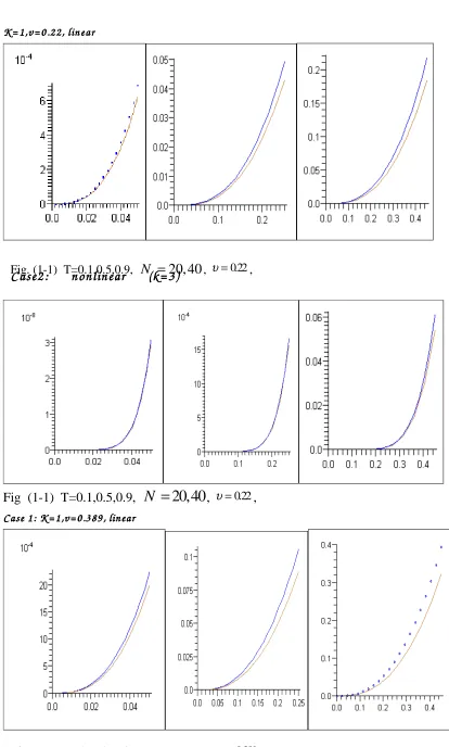
N = , which it represented in the following Table 1, and plot the error ΕN as shown in Figs. [(1-1) - (1-6)].

S I J E N

IJENS © December 2011 IJENS

-IJBAS 9494 -06 46 11

T N

t Exact

linear k=3 linear k=1

Polyurethane

v=0.389 Nickel _v=.28

Polyurethane

v=0.389 _v=.28 Nickel

Approximate error

Approximate error

Approximate

error

Approximate error

0.1 20

2.00000E-02 4.00000E-04 4.00000E-04 1.30000E-12 4.00000E-04 3.00000E-13 4.03078E-04 3.07757E-06 4.00080E-04 8.28887E-08

4.00000E-02 1.60000E-03 1.60000E-03 3.10000E-11 1.60000E-03 4.00000E-12 1.62185E-03 2.18465E-05 1.60058E-03 5.79920E-07

8.00000E-02 6.40000E-03 6.40000E-03 5.88000E-10 6.40000E-03 9.00000E-11 6.55504E-03 1.55043E-04 6.40396E-03 3.95932E-06

1.00000E-01 1.00000E-02 1.00000E-02 1.48000E-09 1.00000E-02 2.29000E-10 1.02945E-02 2.94518E-04 1.00074E-02 7.35131E-06

40

2.00000E-02 4.00000E-04 4.00000E-04 2.00000E-13 4.00000E-04 1.00000E-13 4.02078E-04 2.07830E-06 4.00052E-04 5.23491E-08

4.00000E-02 1.60000E-03 1.60000E-03 6.00000E-12 1.60000E-03 0.00000E+00 1.61411E-03 1.41085E-05 1.60035E-03 3.54479E-07

8.00000E-02 6.40000E-03 6.40000E-03 1.05000E-10 6.40000E-03 1.50000E-11 6.49837E-03 9.83678E-05 6.40240E-03 2.39963E-06

1.00000E-01 1.00000E-02 1.00000E-02 2.58000E-10 1.00000E-02 3.60000E-11 1.01861E-02 1.86119E-04 1.00044E-02 4.45052E-06

0.5 20

1.00000E-01 1.00000E-02 1.00000E-02 6.16000E-09 1.00000E-02 1.15000E-09 1.09863E-02 9.86296E-04 1.00231E-02 2.30943E-05

2.00000E-01 4.00000E-02 4.00001E-02 7.23600E-08 4.00000E-02 1.24100E-08 4.84412E-02 8.44119E-03 6.27345E-04 1.65880E-04

4.00000E-01 1.60000E-01 1.60014E-01 1.40604E-05 1.60000E-01 7.38000E-07 2.52379E-01 9.23792E-02 1.61192E-01 1.19223E-03

5.00000E-01 2.50000E-01 2.50165E-01 1.64587E-04 2.50000E-01 7.41580E-06 4.73773E-01 2.23773E-01 2.52269E-01 2.26860E-03

40

1.00000E-01 1.00000E-02 1.00000E-02 6.80000E-10 1.00000E-02 2.24500E-09 1.05633E-02 5.63321E-04 1.00143E-02 1.42556E-05

2.00000E-01 4.00000E-02 4.00000E-02 1.18800E-08 4.00000E-02 1.32000E-09 4.45750E-02 4.57502E-03 4.00994E-02 9.93666E-05

4.00000E-01 1.60000E-01 1.60010E-01 9.93120E-06 1.60000E-01 4.21100E-07 2.06464E-01 4.64636E-02 1.60709E-01 7.08539E-04

5.00000E-01 2.50000E-01 2.50115E-01 1.15030E-04 2.50005E-01 4.63510E-06 3.57887E-01 1.07887E-01 2.51347E-01 1.34655E-03

0.9 20

1.80000E-01 3.24000E-02 3.24003E-02 3.01090E-07 3.24001E-02 9.82000E-09 4.46008E-02 4.46008E-02 3.25882E-02 1.88189E-04

3.60000E-01 1.29600E-01 1.29608E-01 7.74750E-06 1.29601E-01 8.66200E-07 2.72550E-01 1.42950E-01 1.30983E-01 1.38313E-03

7.20000E-01 5.18400E-01 5.44479E-01 2.60787E-02 5.19005E-01 5.19005E-01 4.41743E+00 3.89903E+00 5.28821E-01 1.04207E-02

9.00000E-01 8.10000E-01 1.67415E+00 2.48415E+00 8.19195E-01 9.19473E-03 1.76509E+01 1.68409E+01 8.30301E-01 2.03013E-02

Table (1)

Fig. (1-1) T=0.1,0.5,0.9, N =20, 40, υ=0.22, k=1.

7.20000E-01 5.18400E-01 5.32880E-01 1.44801E-02 5.18784E-01 3.83681E-04 1.54445E+00 1.02605E+00 5.24481E-01 6.08105E-03

9.00000E-01 8.10000E-01 3.06363E+00 3.87363E+00 8.15351E-01 5.35145E-03 4.26984E+00 3.45984E+00 8.21824E-01 1.18242E-02

Fig. (1-2) T=0.1,0.5,0.9, N =20, 40, υ =0.22_, Case3

Case3 Case3

Case3 : linear (k= 1), v=0.389: linear (k= 1), v=0.389: linear (k= 1), v=0.389 : linear (k= 1), v=0.389

C ase4:

C ase4: C ase4:

C ase4: nonlinear (k= 3), v= 0.389nonlinear (k= 3), v= 0.389nonlinear (k= 3), v= 0.389 nonlinear (k= 3), v= 0.389

Fig.(1-3)T=0.1,0.5,0.9, N =20, 40,υ=0.389,

C ase C ase C ase

C ase2222: nonlin ear (k= 1) v=0.22: nonlin ear (k= 1) v=0.22: nonlin ear (k= 1) v=0.22 : nonlin ear (k= 1) v=0.22

A A A

A p plication 2 p plication 2 p plication 2 p plication 2

If the kernel of the NVEE of the second kind can be represented in the logarithmic kernel k t x( , )=lnt −x , we get

( )

( )

( )

0

ln , 1

t

k

t t x x dx f t k

µθ

−

λ

_∫

−

θ

= > , (5.3)

when k = 1, Eq. (5.3) reduces to linear Volterra integral equation of the second kind

( )

( )

( )

0 ln

t

t t x x dx f t

µθ

−

λ

_∫

−

θ

= . (5.4)

The N um erical results : The N um erical results : The N um erical results : The N um erical results :

In Table 2, we use Maple programm to compute the exact and approximate solutions and the errors ΕN of Eq .(5.3) , (5.4) with logarithmic kernel numerically by using the product Nyström method , for linear (k =1) and nonlinear (k = 3) cases, , for different

values of

υ

= 0.389 and 0.22, that corresponding to Polyurethane and Nickel materials at T= 0.1, 0.5 ,0.9, and N =20, 40,. Also,

the error ΕN is plotted as shown in Figs. (1-7) -(1-12)

T N

t Exact

linear k=1 linear k=3

Polyurethane material v=0.389,

λ

=

Nickle material v=.28,

λ

=

Polyurethane material v=0.389,

λ

=

Nickle material v=.28,

λ

=

Approximate

so. Error

N

Ε Approximate _sol. Error ΕN Approximate _sol. Error ΕN Approximate _Sol. Error ΕN

0.1 20

2.00000E-02 4.00000E-04 3.75250E-04 2.47503E-05 3.90392E-04 8.36681E-06 4.00000E-04 1.80000E-12 4.00000E-04 6.00000E-13

4.00000E-02 1.60000E-03 1.42194E-03 1.78063E-04 1.52546E-03 6.51476E-05 1.60000E-03 2.33000E-10 1.60000E-03 8.40000E-11

8.00000E-02 6.40000E-03 5.17866E-03 1.22134E-03 5.83675E-03 4.95174E-04 6.39997E-03 2.92070E-08 6.39999E-03 1.06070E-08

S I J E N

IJENS © December 2011 IJENS

-IJBAS 9494 -06 46 11

40

2.00000E-02 4.00000E-04 3.79545E-04 2.04550E-05 3.91633E-04 9.60782E-06 4.00000E-04 8.00000E-13 4.00000E-04 2.00000E-13

4.00000E-02 1.60000E-03 1.44716E-03 1.52841E-04 1.53485E-03 7.45390E-05 1.60000E-03 1.97000E-10 1.60000E-03 7.10000E-11

8.00000E-02 6.40000E-03 5.31875E-03 1.08125E-03 5.90483E-03 5.63247E-04 6.39997E-03 2.74260E-08 6.39999E-03 9.96000E-09

1.00000E-01 1.00000E-02 8.00273E-03 1.99727E-03 9.05602E-03 1.07108E-03 9.99987E-03 1.31647E-07 9.99995E-03 4.78140E-08

0.5 20

1.00000E-01 1.00000E-02 8.35596E-03 1.64404E-03 9.23824E-03 7.61760E-04 9.99989E-03 1.09366E-07 9.99996E-03 3.57030E-08

2.00000E-01 4.00000E-02 2.95785E-02 1.04215E-02 3.44464E-02 5.55362E-03 3.99867E-02 1.32824E-05 3.99952E-02 4.82935E-06

4.00000E-01 1.60000E-01 9.89625E-02 6.10375E-02 1.22025E-01 3.79752E-02 1.58443E-01 1.55743E-03 1.59419E-01 5.81316E-04

5.00000E-01 4.00000E-04 1.44011E-01 1.05989E-01 1.80686E-01 6.93144E-02 2.43195E-01 6.80519E-03 2.47339E-01 2.66089E-03

40

1.00000E-01 2.50000E-01 8.82208E-03 1.17792E-03 9.38792E-03 6.12078E-04 9.99990E-03 9.76780E-08 9.99996E-03 3.54840E-08

2.00000E-01 0.00000E+00 3.19828E-02 8.01721E-03 3.54670E-02 4.53301E-03 3.99882E-02 1.18472E-05 3.99957E-02 4.30840E-06

4.00000E-01 4.00000E-02 1.09813E-01 5.01867E-02 1.28246E-01 3.17541E-02 1.58560E-01 1.43953E-03 1.59460E-01 5.39581E-04

5.00000E-01 9.00000E-02 1.61172E-01 8.88282E-02 1.91492E-01 5.85077E-02 2.43690E-01 6.30959E-03 2.47509E-01 7.99269E-05

0.9 20

1.80000E-01 1.60000E-01 2.61072E-02 6.29280E-03 2.89257E-02 3.47434E-03 3.23942E-02 5.78576E-06 3.23979E-02 2.10291E-06

3.60000E-01 2.50000E-01 8.99749E-02 3.96251E-02 1.05111E-01 2.44890E-02 1.28921E-01 6.79053E-04 1.29349E-01 2.51254E-04

7.20000E-01 1.29600E-01 2.90517E-01 2.27883E-01 3.58285E-01 1.60115E-01 4.69716E-01 4.86837E-02 4.93993E-01 2.44069E-02

9.00000E-01 2.91600E-01 4.16235E-01 3.93765E-01 5.22180E-01 2.87820E-01 6.87619E-01 1.22381E-01 7.27450E-01 8.25497E-02

1.80000E-01 5.18400E-01 2.79278E-02 4.47222E-03 2.97376E-02 2.66238E-03 3.23950E-02 5.04220E-06 3.23982E-02 1.83260E-06

3.60000E-01 8.10000E-01 9.99744E-02 2.96256E-02 1.10349E-01 1.92508E-02 1.29009E-01 5.90666E-04 1.29381E-01 2.19227E-04

7.20000E-01 3.24000E-02 3.35933E-01 1.82467E-01 3.87667E-01 1.30733E-01 4.76825E-01 4.15754E-02 4.96709E-01 2.16909E-02

9.00000E-01 1.29600E-01 4.87577E-01 3.22423E-01 5.71650E-01 2.38350E-01 7.10396E-01 9.96044E-02 7.37991E-01 7.20088E-02

K = 1,v=0.22, linear K = 1,v=0.22, linear K = 1,v=0.22, linear K = 1,v=0.22, linear

Fig (1-1) T=0.1,0.5,0.9,

N

=

20,40

, υ=0.22, Case 1: K =1,v=0.389, linear

Case 1: K =1,v=0.389, linear Case 1: K =1,v=0.389, linear Case 1: K =1,v=0.389, linear

C ase2:

nonlinear

(k= 3)

C ase2:

nonlinear

(k= 3)

C ase2:

nonlinear

(k= 3)

C ase2:

nonlinear

(k= 3)

Case 2: Case 2: Case 2:

Case 2: K =3,v=0.389K =3,v=0.389K =3,v=0.389 , nonlinearK =3,v=0.389, nonlinear, nonlinear, nonlinear

Conclusions

Conclusions Conclusions Conclusions

In general, from the previous results in Tables (1)-(2), we deduce the following discussions:

1) For linear (k =1) and nonlinear (k =3) VIE, the result error ΕN decrease as well as the values of N increases for different values of

υ

,

λ

.

2) For different values of

υ

,

λ

, in the linear (k =1) and the nonlinear (k =3) cases , the result errors ΕN of the product Nyström method with Carleman kernel is less than the ΕN with logarithmic kernel, as shown in Tables 1,2. 3) The error ΕN is increases as well as the value of time T tends to unity for all

different values of

υ

,

λ µ

, . Also, the error ΕN is increases as well as the value of t increasing for t∈[0,0.1], t∈[0,0.5] and t∈[0,0.9].

4) The error ΕN for linear case are larger than nonlinear case, for different values of

υ

and

λ

, k .

5) Due to the kernel of Carleman , as the values of

υ

is increasing i.e.(0< <

υ

0.4), the values of errors ΕN are also increasing for T = 0.1 0.5, 0.9

6) Due to the logarithmic kernel, as the value of

λ

is increasing (0< <

υ

0.4), the value of error is also increasing for T = 0.1 0.5.

7) Due to the kernel of Carleman, if the value of parameter

υ

tends to one, i.e. (0.4≤ <

υ

1) (i.e. the materials is solid). and the time T also tends to unity i.e. T= 0.9, then the resultant errors ΕN are greater than 1 ( i.e. the numerical solutions farmer than the exact solutions) .

R eferences R eferences R eferences R eferences

[1] C.D. Green , Integral Equation Methods , Nelson , New York , 1969

[2] H. Hochstadt , Integral Equations , A wiley Inter Science Publication, New York , 1973.

[3] R.P. Kanwal, Linear Integral Equations Theory and Technique, Boston , 1996. [4] P . Schiavone , C.Constanda and A. Mioduchowski , Integral Methods in Science and Engineering , Birkhauser Boston, 2002.

[5] N. I. Muskelishvili , Singular Integral Equations, Noordhoff, 1953.

[6] N. I. Muskhelishvili, Some Basic problems of Mathematical Theory of Elasticity, Noordhof, Holland, 1953.

[7] J, Abdalkhani, A numerical Approach to the Solution of Abel Integral Equation of the Second Kind with nonsmooth solution , J.Comput. Appl. Math. 29, 249-355 (1990). [8] H. Guoqiang, K. Hayami, K. Sugihura, and W. Jiong ,Extrapolation Method of Iterated collocation Solution of Tow Dimensional Nonlinear Volterra Integral

Equation, J. Appl. Math. Comput. 112, 49-61 (2000).

[9] H. Brunner, M. R. Crisci, E. Russo and A. Recchio, A family of Methods for Abel Integral Equations of the Second Kind, J. Comp. Appl. Math. 34. (1991),211-219.

[10] J. P. Kauthen, A survey of Singular Perturbed Volterra Equations. Appl. Num. Math. 24, (1997). 95-114.

[11] A. A. kilbas and M. Saigo, On Solution of Nonlinear Abel-Volterra Integral Equation, J. Math. Ahaly. Appl. 229, (1999).41-60.

[12] A. P. Orsi, Product Integration for Volterra Integral Equations of the Second Kind with Weakly Singular Kernels, Math. Comp. Vol 56(216). (1996) 1201-1212.

[13] Lu Tao, Huang Young, Extrapolation Method for Solving Weakly Singular Nonlinear Volterra Integral Equations of the Second Kind, J. Math. Anal. Appl. 324, (2006). 225-237.

[14] Badr, A. A. “On some parameter methods for nonlinear volterra intogral equation, “App. Math. Comp. 117(2001)15-22.

[15]Peter Linz, Analytic and Numerical Methods for Volterra Equations, Siam, Philadelphia, 1985.