Characterization and Performance Analysis for 3D Benchmarks

Characterization and Performance Analysis for

3D Benchmarks

Joseph Issa

Santa Clara University

Department of Computer Engineering, 500 El Camino Real, Santa Clara, CA 95053, USA Email: jissa@scu.edu

Abstract— The change in processor architectures and 3D

benchmarks makes performance characterization important for every processor and 3D application generation. Recent 3D applications require large amount of data to be processed by the GPU and the CPU. This leads to the importance in analyzing processor performance for different architectures and benchmarks so that benchmarks and processors are fine-tuned to achieve better performance. In this paper, we propose a performance analytical model for the CPU and the GPU. The analytical model takes different architecture as input parameters to estimate performance. We used two different 3D applications, Crysis game and 3DMarkVantage. We characterize both benchmarks for performance bottlenecks and propose an analytical model to estimate performance at different configurations with error deviation <5%.

Index Terms— performance characterization, performance

measurement, performance analysis, performance modeling

I. INTRODUCTION

For every set of new processors released, a new set of workloads are also released that are used to rank the processor’s performance. Most of these new benchmarks require a considerable amount of computational power. Processor designers usually trail the new release of benchmarks to set ahead the expected performance for specific processor designs on specific workloads, which enables them to project performance for their new architecture before doing actual performance measurements. There are several fundamental differences between CPU and GPU. CPUs can provide faster response time for a single task; this is due to several architectural changes that can improve performance. These architectural features can improve performance but comes at the expense of higher power budget cost. GPUs are designed for graphics application purposes. During rendering process, the time latency to process one pixel by GPU may not be very critical assuming other pixels can be rendered separately before completing one frame. This leads us to the importance of analyzing and predicting performance for GPU as well as CPU for 3D applications. Predicting processor performance on a given workload is a key to fine-tuning current designs to achieve higher performance scores. The characterizations of the workload and processor architecture are keys to achieving an

accurate baseline so that any performance prediction from that baseline will have minimum error deviation from actual measurements. There is extensive literature on CPU performance prediction for different workloads [25][26], but there are few papers published on performance prediction analytical models based on measurements and simulation-based analysis for GPU and CPU using 3D benchmarks. This is partly because processors and 3D benchmarks continue to change their programming methods and architectures. Analyzing the amount of work to process by the CPU for these 3D applications and projecting performance for both GPU and CPU are essential for any processor and workload developer for fine-tuning their current design’s by understanding performance bottlenecks, architecture sensitivity, and enabling designers to project performance for different processor architecture without measurements. For the GPU, we used Amdahl’s Law analytical model to project GPU performance from a measured baseline, while on CPU, we used simulation baseline analysis for different architecture variables and applied Amdahl’s Law to project for different processor configurations (i.e., CPI scaling). The goal of this paper is to analyze and characterize a set of recent interactive 3D games and benchmark at the microarchitecture level. The remainder of the paper is organized as follows: Section II discusses related work, Section III derives the Amdahl’s Law method, and section IV discusses benchmark selection. In section V, we apply the performance prediction method for GPU architecture. In Section VI discusses traces selection method and applies Amdahl’s Law to estimate performance and we conclude in section VII.

II. RELATED WORK

project performance on different workloads and different processor architectures for both the CPU and GPU.

Saavedra [9] used program execution for a given benchmark to characterize both machine performance and program execution. His scheme focuses on total execution time for a given benchmark. The difference between the method proposed in this paper and the method proposed in [9] is that our method is generic and be used for any processor and benchmark. Our method also can project the maximum performance a benchmark can achieve for a processor under test as well as project for different processors of the same family architecture.

Krishnaprasad [10] describes different methods for using Amdahl’s Law in different forms, but his paper does not describe how to implement Amdahl’s Law in a recursive form as described in our method.

Hoste [11] computes the set of micro-architecture independent characteristics and weights these independent characteristics, resulting in locating the application of interest in benchmark space. Performance is predicted by weighting the performance number of a benchmark in the neighborhood of application of interest. This method might be close to our trace weighting method and workload characterization except that it does not present a performance prediction method.

Roca [31] presented detailed 3D workload characterizations for CPU and GPU based on trace simulations and analysis. The paper does not include performance prediction method for different processor architectures.

III. AMDAHL’S LAW OVERVIEW

The prediction method derived in this paper is based on Amdahl’s Law method in which we modified the existing law and applied it in a recursive form. In this model, we refer to two domains: the time domain and the score domain. The time domain is inversely proportional to the score domain. After deriving the projected linear equation line in the time domain, we will convert it to the score domain so we can project performance for a given benchmark. Our approach projects processor performance for a graphics processor on a given benchmark by implementing the following steps:

First, we establish a measured baseline for a given graphics processor by taking a minimum of two measured data points. These two measured data points can be memory frequencies, core frequencies, or two different GPUs of similar architecture but with different number of core. The measurement in this case is performance data for two different numbers of cores.

Second, determine the scaling and non-scaling variables to plot the score line that will be used for prediction. The scaling and non-scaling variables in this paper are referred to as a and b variables, respectively. These two variables used to determine the characteristics of the linear prediction in the time domain, as well as to determine the maximum performance a graphics processor can achieve for the benchmark selected in step 1 in the score domain, by taking the inverse of non-scaling variable b.

Third and finally, using the score line derived in step 2, we can now project for a different graphics processor of the same architecture as that used in step 1. The method defined in this paper is limited to projecting performance for similar graphics processor architecture. The basic for Amdahl’s Law [3,4] states that the performance improvement to be gained from using some faster mode of execution is limited by the fraction of the time the faster mode can be used. In other words, the system’s overall performance increase limited by the fraction of the system that cannot take advantage of the enhanced performance. Therefore, the performance of a system divided into two distinct categories: the part that improves with the performance enhancement and is said to scale (variable a), and the part that does not improve due to the performance enhancement and is said to not scale or to be non-scaling (variable b).

Amdahl’s law takes the algebraic form

(

)

0 1 0 .

f

T T T T

f

= + − (1)

Where T1 is the measured execution time at frequency f1

and T0 is the non-scale time. Note that Amdahl’s law if a function of frequency and time, it does not take any architectural variable in account such as different number of cores.

We can write T0 in terms of a second measurement T2 at f2:

2 2 1 1

. 0

2 1

T f T f

T

f f

− =

− (2)

When we substitute Equation (2) for T0, we obtain Amdahl’s law in terms of two specific measurements without reference to T0:

1

( )

,

T

a

b

f

=

+

where

2 2 1 1

2 1

,

f T

f T

a

f

f

−

=

−

and

1 2 1 2

2 1 .

T T

b f f

f f

⎛ − ⎞

= _{⎜ ⎟}

−

⎝ ⎠

(5)

Variables a and b can be transformed to the score domain using S ≡ 1/T. For two data points, we will have (f1,S1) and (f2,S2), and for n data points, we will have (f1,S1), …, (fn,Sn). We expect these points to satisfy an equation of the form (except for noise):

,

f

i

S

i

_{a f}

_b

i

≈

⋅ +

obtain best estimates for a and b. In particular, given a and b, we take the error in our estimate for Si in terms of fi

to be the difference between the measured and estimated value for Si. The best estimates for a and b are those that

minimize the sum of the squares of these errors:

2

1

n

i i

E

e

=

=

∑

The estimates for a and b are those at which the values of the partial derivatives ∂E/∂a and ∂E/∂b are simultaneously zero. By computing these derivatives explicitly, we obtain equations satisfied by the best choices for a and b, which is the best functional fit to the measured data.

If the data points are in the Time Domain (f1,T1), …, (fn,Tn), we can use the relationship of score to time, and determine the best estimate for T in terms of f .

Evaluating the equations, we can derive a and b in terms of T and f for n points. We can also calculate a and b values to construct the linear score line in terms of S1, S2, f1 and f2 by substituting S ≡ 1/T in the a and b equations.

IV. BENCHMARKS SELECTION

Benchmark selections for Crysis[2] game and 3DMarkVantage[1] are based on different criteria, such as DX support and popularity for performance measurements that provide different benchmark test suites that involve CPU and GPU workloads. Crysis game is a first-person shooting game that comes with an integrated benchmark test suite with DX9 and DX10 support. The measured metric for Crysis performance is frames-per-second. For 3DMarkVantage, it covers graphics tests as well as CPU tests by providing two different benchmark CPU tests, where CPU Test #1 features a high-intensity workload of co-operative path-finding artificial intelligence calculations. This workload can utilize multi-core CPUs, while CPU Test #2 features a heavy physics workload. The performance metrics measured for CPU Test #1 is in plans/sec and for CPU Test #2 is in steps/sec. Since most of the rendering is processed by the GPU, the CPU is still doing the intelligence, physics tests, and other calculations required for the workload. In this paper, we analyze both aspects of the benchmark for the CPU and the GPU. For GPU performance predictions, we use Amdahl’s Law to project performance from a measure baseline, while for CPU, we use simulation baseline and apply Amdahl’s Law to project for different processor architectures.

V. GPU PERFORMANCE ANALYSIS

The experimental results discussed in this section are GPU based on applying Amdahl’s Law method. The process of GPU performance prediction for 3D games entails three steps. The first step is to determine what to project, for example for higher core frequency, or higher memory frequency, or higher number of cores on a target graphics card of the same architecture. The second step

involves establishing a measured baseline to project from while keeping all other variables but one fixed (i.e. core frequency is a variable while the number of cores and memory frequency/bandwidth are fixed). The third step is to project for a target processor of the same architecture.

A. Performance Analysis for GPU Memory Frequency Using Crysis 3D Game

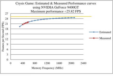
The prediction method requires a minimum of two measured points for a given benchmark to establish the baseline for prediction. In our first experiment, we use the Crysis game with resolution 1024x768 with NVidia GeForce 9400GT [5] graphics card. We measured two data points at different memory frequencies while keeping the core frequency fixed, so the only variable we project is the memory frequency. The model requires at least two measured data points at two different frequencies, the more data points we measure the better in terms of minimizing the prediction error. However, in this paper we will use two measured data points for all out measured baselines. The two measured points for Crysis game memory frequency are as follows: Measured point #1: Memory Frequency@400 MHz, Frames per Second (FPS) ~ 20; measured point #2: Memory Frequency@450 MHz, FPS ~21. Using these two measured data points as the input baseline to our prediction module, the method will project Frames per Second (FPS) score for the remaining memory frequencies without any measurement. Figure 1 shows the memory prediction curve based on the two measured points we have. For this experiment, the a and b values are the prediction line intercept and slope values that are calculated as 3.9101 and 0.0387, respectively, to form the equation y=ax+b. At x=0 and y=0.0387, it is the non-scaling part of the equation.

Figure 1: Memory frequency performance curve based on NVidia 9400 GT.

From the derived equation y=3.9101x+0.0387 at x=0, y=0.0387. Taking the inverse of y, 1/y=1/0.0387=25.8, this result for 1/y concludes that the score (FPS) will never exceed ~ 25 FPS as memory frequency increases. To illustrate, we used the same two data points we have measured before for the Crysis game to establish the baseline. Then projecting frames per second at high memory frequencies, we noticed that at high memory frequencies, the performance curve remains flat, as shown

0 3 6 9 12 15 18 21 24 27

0 400 800 1200 1600 2000 2400

F

rames

per Second (F

PS)

Memory Frequency (MHz)

Crysis Game: Estimated & Measured Performance curves using NVIDIA GeForce 9400GT Maximum performance =25.82 FPS

Estimated

in Figure 1. Hence, y is the non-scaling coefficient for this data set. The maximum performance is bounded by an upper limit of 1/Y. The actual NV 9800GT GPU control utility provided by NVidia will not allow setting memory frequencies more than it can handle. Therefore during measurements, we could not set the memory frequency higher than 900 MHz, which is why we need to project for performance at higher memory frequencies so we can project for a different graphics card of the same architecture that can support higher memory frequencies compared to the NV 9400GT[5] card.

B. Performance Analysis for GPU Core Frequency using Crysis 3D Game

In the next experiment, we used the same Crysis game, but with an ATI HD3470 [6] graphics card. Now, instead of projecting for performance at different memory frequencies, we project for performance at different core frequencies. Following the same steps we used for memory frequency prediction, we took two data points measured as follows: Measured point #1: GPU Core Frequency @300MHz FPS ~ 6; measured point #2: GPU Core Frequency @400MHz, FPS ~ 8. From the two measured data points, we use the prediction method and plot the prediction curve for GPU frequency as shown in Figure 2.

Figure 2: Performance estimate curve for GPU core frequency scaling based on ATI HD3470.

In addition to the two measured data points, we took several measured data points up to 700MHz, as shown in in Figure 2 (marked ‘Measured’). The prediction module also calculates the a and b values to plot the linear score line. We followed the method used before to calculate maximum performance. The linear score equation for the ATI HD3470 [6] is y=43.372x+0.0104. x=0, y=0.0104, and 1/y = 96.15 FPS, although in reality, the graphics card can never achieve this frequency and the utility provided by ATI to override the core frequency will not allow core frequency to be set to more than the processor can handle. Again, the reason we calculate it is to be able to use this projected data for other cards of the same architecture that may achieve higher core frequency compared to the HD3470. The maximum performance upper-bound maximum limit at ~ 92 FPS as shown in Figure 3.

Figure 3: Core frequency estimated curve based on ATI HD3470.

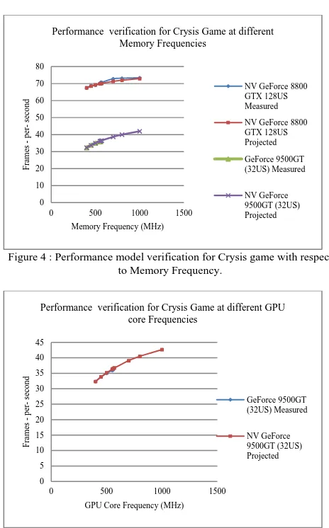
We verified the prediction model for different NVidia graphics cards with respect to GPU core and memory frequency scaling as shown in Figure 4 and Figure 5. We show projected versus measured data in which the error deviation is < 5% in all cases.

Figure 4 : Performance model verification for Crysis game with respect to Memory Frequency.

Figure 5: Performance model verification for Crysis game with respect to GPU core Frequency.

We also calculated the a and b parameters to determine the slope and intercepts of the linear performance line

0.0 5.0 10.0 15.0 20.0 25.0 30.0 35.0 40.0 45.0

0 1000 2000 3000 4000

F

rames

per Second (F

PS)

GPU Frequency (MHz)

Crysis Game: Estimated & Measured Performance curves using ATI HD 3470

Estimated

Measured

0.0 10.0 20.0 30.0 40.0 50.0 60.0 70.0 80.0 90.0 100.0

0 10000 20000 30000 40000 50000 60000

F

rames

per Second (F

PS)

GPU core Frequency (MHz)

Crysis Game: Estimated & Measured Performance curves for ATI HD 3470 at High core frequencies

Estimated

Measured

0 10 20 30 40 50 60 70 80

0 500 1000 1500

Fram

es

-p

er-second

Memory Frequency (MHz)

Performance verification for Crysis Game at different Memory Frequencies

NV GeForce 8800 GTX 128US Measured NV GeForce 8800 GTX 128US Projected GeForce 9500GT (32US) Measured

NV GeForce 9500GT (32US) Projected

0 5 10 15 20 25 30 35 40 45

0 500 1000 1500

Fram

es

-p

er-second

GPU Core Frequency (MHz)

Performance verification for Crysis Game at different GPU core Frequencies

GeForce 9500GT (32US) Measured

equation. The theoretical maximum performance score as frequency increases to much higher values are shown in

错误！未找到引用源。.

TABLE I.

CRYSIS MAXIMUM PERFORMANCE FOR MEMORY AND GPU CORE FREQUENCIES FOR DIFFERENT NV CARDS.

Configuration Intercept slope Frequency

scaling

Maximum performance NV GeForce 8800

GTX 128 CUDA Cores

0.01298 0.73 Memory 77 FPS

NV GeForce 8600GTS 32 CUDA Cores

0.02033 4.43 GPU 49.188 FPS

NV GeForce 9500GT 32 CUDA Cores

0.01847 4.985 Memory 54.14 FPS

The Crysis game performance scales better with respect to GPU frequency as compared to Memory frequency. There is scaling with respect to memory frequency increase, but not at the ratio compared to GPU core frequency increase. This is shown in Figure 6 were we show measurements for different NVidia card at different memory frequencies, the performance changes at lower rate as memory frequency increases and for some graphics cards there is no change in performance.

Figure 6: Crysis game memory frequency scaling measurements for different NVidia graphics cards.

C. Performance Prediction for A Higher Number of Cores Using 3DMarkVantage Benchmark

For the 3DMarkVantage benchmark, we implemented the same prediction method we used for the Crysis game. However, in this experiment, we have three different ATI discrete cards of the same architecture but with a different number of cores and memory bandwidth. The goal is to be able to project the 3DMarkVantage score for ATI HD4890 [7], and we compared the projected data to measured data for ATI HD4890. We adjusted memory frequency for HD4670 [8] and HD4830 [7] so they can both have the same memory bandwidth while keeping core frequencies the same. This will eliminate the memory bandwidth and core frequency variables in our prediction.

First, we establish the measured baseline using ATI HD4670 [8] and ATI HD4830 [7] graphics cards to project for ATI HD4890 graphics card. The number of cores for HD4670 is equal to 320, and for HD4830 is equal to 640. The goal is to project for HD4890 at 800 cores. Note that all three cards have the same architecture.

Before taking any measurements, we adjusted the core frequency and memory bandwidth to be the same for HD4670 and HD4830. For our experiment, we used core frequency =750 MHz and memory bandwidth ~57 GB/s, by adjusting the memory frequency.

Figure 7: 3DMarkVantage scores for projected versus measured for different ATI graphics cards.

In Figure 7, the measured score for ATI HD4670 is 2237, for ATI HD4830 is 4044. Using these two data points, we implement the prediction method to project for ATI HD4890 at 800 cores; the estimated graphics score is equal to 4823. Next, we measure the actual ATI HD4890 graphics card to compare measured versus projected data under the same settings we used for the prediction. The graphics score measured for ATI HD 4890 card is equal to 4640. The delta error difference between measured (4640) and projected (4823) for ATI HD4890 is ~4%, which meets our objective of < 10% error difference between measured and projected data. Note that the implementation for this experiment is different from the Crysis game [2] experiment implementation because we are utilizing two different graphics cards to be able to project for the third card of the same architecture, but the prediction method is the same for both experiments.

D. Additional Workload to Verify Predition Model We selected additional 3D game Company of Heroes (COH) to verify Amdahl’s law method. COH is a 3D DX10 games, we used ATI HD5670 [32] as baseline for our measurements. This experiment is to verify the method additional to Crysis and 3DMarkVantage workloads. We will not do in-depth analysis for COH like Crysis and 3DmarkVantage. We used Amdahl’s law method derived in this paper; the average error between projected and measured is 1.24% as shown in Figure 8.

0 10 20 30 40 50 60 70 80

0 500 1000 1500

Cr

y

sis F

P

S

Memory Frequency (MHz)

Crysis performance measurments at different Memory Frequencies

NV GeForce 8800GTX NV GeForce 9400GT NV GeForce 9500GT NV GeForce 8600 GTS ATI HD 3450 ATI HD 3470 ATI 2900XT

2237

4044

4640 4823

0 1000 2000 3000 4000 5000 6000

ATI HD4670-320 cores (Measured)

ATI HD4830-640 cores (Measured)

ATI HD4890-800 cores (Measured)

ATI HD4890-800 cores (Estimated)

Tota

l Sc

or

e

Figure 8: COH game performance Analysis.

VI. CPU PERFORMANCE ANALYSIS

Most of the rendering for a 3D application processed by the GPU, but some of the computations are processed by the CPU such as physics and other coordinates calculation. In this section, we will present a CPU tracing analysis and performance estimation based on CPI scaling for Crysis and 3DMarkVantage. For the Crysis game, we traced ~30 CPU-based traces; the platform configuration used for tracing is with CPU at 1400 MHz, 100 MHz Front Side Bus (FSB), NV8800 graphics cards, and 2 GB of RAM. Each trace consists of about 25 million instructions, so we simulate several million instructions instead of simulating the entire workload, which is very time consuming. A trace weight tool is used to determine the weights for each trace. This is done based on six different vectors associated with each trace. Each of these set of traces is simulated with respect to a specific processor configuration such as number of cores, memory size, and memory type and core frequency. For each trace, we used a profiling tool to calculate certain architecture metrics that affect performance for each trace such as CPI, branches miss-prediction, and last level cache miss. The profiling data is than mined for each trace point offset and length to determine each trace point’s vector. The vectors are normalized in each dimension using standardization. Weight for each trace point (in terms of instructions represented or Ireps) calculated by summing the instructions of the associated sample set. The overall performance (time in cycles) of a set of k trace points is:

1

(sec)

( )* ( )*

,

k

i

Total execution time

I i CPI i Weights

Frequency

=

=

∑

(8)

sec *

Instructions per ond =Weighted IPC Frequency

,

(9)

and

1

( ) / ,

k

i

Weighted IPC I Weights i Cycles

=

=

∑

(10)

CPI(i) is the results from simulation of the trace and Irep is the instruction representation for a given trace as

shown in Figure 9. The objective is to set up at least two simulation data points (instead of measured) so we can use them as a baseline and apply the Amdahl’s Law method derived earlier to project for different processor architectures and configuration. We use the weights for the traces when simulating those traces for given processor configuration. Thus, we can map the traces back to the entire workload.

Figure 9: CPI values for all Crysis CPU based samples

The % instruction weight in referred to as the fraction of Irep for a given trace by total Irep is the % weight of each trace relative to the entire Crysis workload. Some traces have more weights compared to other as shown in Figure 10.

Figure 10: Sample weights for Crysis.

The summation of all weights for all traces is equal to 100%. The total number of cycles contributing to the CPI consists of several architecture-dependent cycles that the simulator generates with respect to specific processor configuration. In general, the total cycle is a summation of cycles contributed from conditional branch miss-prediction, conditional branch retired, L2 hits/miss, and other parameters.

A. Sensitivy Analysis Relative to CPI

We use the simulator to run the same set of traces against different processor configurations. The processor configurations selected based on core frequency, number of cores, memory frequency, and cache size. The simulator runs every trace against the processor

0 5 10 15 20 25 30 35 40 45 50

0 500 1000 1500 2000 2500

C

OH-FP

S

Memory Frequency (MHz)

COH- Projected vs. Measured for # of cores =24 , Average Error=1.242% between measured and prediction model

Model

Measured

0 0.5 1 1.5 2 2.5 3 3.5 4

1 2 3 4 5 6 7 8 9 1011 1213 14 15 16 1718 19 2021 22 23 24

CPI

Sample # Crysis CPU - CPI

CPI

0 1 2 3 4 5 6 7 8 9 10

1 3 5 7 9 11 13 15 17 19 21 23

Trace W

ei

g

ht

Sample #

Crysis CPU - %instructions

configuration and generates an output file with details of processor architecture dependencies such as instructions retires, cycles, branch misses, L2 hit/Miss, Last level cache miss, and other architecture variables. For our analysis in this paper, we look at CPI (Cycles-Per-Instruction) which is an important performance parameter.

As discussed before, 3DMarkVantage offers CPU Test#1 and Test#2 are part of the benchmark test suite. CPU Test#1 is a high-intensity workload of co-operative path-finding artificial intelligence calculations, while CPU Test#2 features a heavy physics workload.

We show that CPU Test#2 is not sensitive to core or memory frequency since the CPI almost is the same, while CPU Test#1 is sensitive to core frequency but not sensitive to memory frequency. The CPI for CPUTest #1 is lower (the lower, the better) for all traces with CPU Frequency at 3300 MHz, Memory Frequency at 1333 MHz, compared to CPU Frequency at 3000 MHz, Memory Frequency at 1600 MHz, while keeping the number of cores and cache size fixed for all configurations.

For the Crysis workload, we selected two processor configurations with the exact same number of cores, frequency, and memory type/frequency and cache sizes. However, these two different processors have different architectures such as buffer sizes and larger queues. The objective for this analysis is to understand performance impact for micro-architectural change on a given processor. The CPI scaling shows significant improvement in performance (lower CPI) for processor architecture #1 for all Crysis traces as shown in Figure 11.

Figure 11: Crysis game CPI variation.

B. Performance Analysis for CPU

After analyzing the benchmark behavior and sensitivity with respect to different processor architectures and configurations, Amdahl’s Law method derived in the previous section is used to project for processor performance. However, in this section, the baseline derived from simulations, not the measured baseline. As discussed before, Amdahl’s Law requires at least two simulated (or measured) data points to project to different processor configurations. The weight associated with each trace is applied by multiplying the weight with CPI for a given trace; the summation will give us the total CPI for

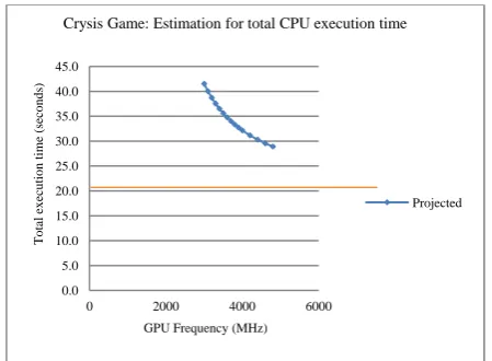
all traces combined, which is expected to have good representation of the entire benchmark. To transfer these results to time (in seconds), the result is divided by the frequency of the processor for each trace. Figure 12 shows the total execution time for all traces combined for different processor configuration.

Figure 12: Crysis total execution time based on sample analysis.

We used Amdahl’s Law by taking two different simulated execution time data points at CPU frequency of 3200 MHz and 3600 MHz. The total execution time (in seconds) projected for all simulated traces at higher core frequency. The total CPU execution time starts leveling off as frequency increases, which is about 22 seconds of total execution time. To confirm this observation, we derive a and b variables using Amdahl’s Law method.

The linear prediction line equation derived is y

=-75.246x+0.0466 at x=0, y=0.0466, taking the inverse of y, 1/y=21.45. This is the lower bound of the total execution time for all the Crysis traces, meaning that no matter how much frequency is increased, the total execution time will never fall below 21.45 seconds as shown in Figure 13.

Figure 13: Crysis execution time prediction curve using simulated time for CPU frequencies 3200 MHz and 3600 MHz as a baseline.

For 3DMarkVantage predictions, we used the same method, but for this benchmark, we project for CPI (the lower, the better the performance) instead of total execution time as we did for Crysis. Since we have CPU Tes#1 and CPU Test#2 workloads in 3DMarkVantage, we project CPI for both. Note that CPU Test#2 CPI does not

0 0.5 1 1.5 2 2.5

0 10 20 30 40

CPI

Sample #

Crysis Game: CPU CPI Analysis

#cores=4, Cache Size=8M, Core Freq=3200MHz, DDR3_1600 (Arch#1)

#cores=4, Cache Size=8M, Core Freq=3200 MHz, DDR3_1600 (Arch#2)

0 5 10 15 20 25 30 35 40 45 50

Processor Configurations

Time

(s

ec

)

Crysis Game: Total Execution Time

#cores=4, Cache Size=8M, Core Freq=3200 MHz, DDR3-1600 (Arch #1) #cores=4, Cache Size=8M, Core Freq=3200 MHz, DDR3_1600 (Arch #2) #cores=4, Cache Size=8M, Core Freq=3200MHz, DDR3_1600 (Arch#1) #cores=4, Cache Size=8M, Core Freq=3600 MHz, DDR3_1600 (Arch#1) #cores=4, Cache Size=8M, Core Freq=3200 MHz, DDR3_1600 (Arch#2) #cores=4, Cache Size=8M, Core Freq=3600 MHz, DDR3_1600 (Arch#2)

0.0 5.0 10.0 15.0 20.0 25.0 30.0 35.0 40.0 45.0

0 2000 4000 6000

Total ex

ecution

time (seconds)

GPU Frequency (MHz)

Crysis Game: Estimation for total CPU execution time

scale as well with processor frequency as CPU Test#1 does. For CPU Test#1 workload, the linear performance equation derived is y = -1166.9x + 0.9984. At x=0, y=0.9984, the inverse of y is 1/y=1.001. This means the CPI for CPU Test#1 will never falls below 1.001 because CPU frequency increases to much higher values >10 GHz. For CPU Test#2 workload, the linear performance derived equation is y = -66.584x + 0.7314. At x=0, 1/y=1.36, so as CPU frequency increases, CPI will never fall below 1.36 for CPU Test#2 workload as shown in Figure 14.

Figure 14: CPI estimate curves for 3DMarkVantage CPU Test#1 and CPU Test#2 workloads.

After analyzing CPI scaling and prediction for 3DMarkVantage CPU Test#1 and CPU Test#2 workloads, we will use a similar method to that we used for Crysis to calculate and project total processor execution time. We use Eq. (9) to calculate total execution time, and applying it to two different processor configurations at 3000 MHz and 3300 MHz processor to get two simulation-based points required for Amdahl’s Law method. The weighted IPC for CPU Test#1 and CPU Test#2 combined is 1.07. The 3DMarkVantage CPU Test#1 and CPU Test#2 final scores calculated as:

3

ec *

, Final Score for DMarkVantage

InstructionsPerS ond CoreFrequency Instructions perOperation

=

(11)

and

, I IPC

Total Cycles

=

∑

(12)

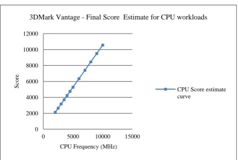
The processor configuration used for this experiment is 3000 MHz core frequency, 6M cache size, and DDR3-1333MHz. Using this baseline, at core frequency 3000 MHz, the combined score for CPU Test#1 and CPU Test#2 is 3171, and for core frequency 3300 MHz the score is 3488. We than use analytical model discussed earlier in this paper to project performance at higher CPU core frequencies as shown in Figure 15.

Figure 15: 3DMarkVantage CPU workload performance curve.

The reason we used trace-based analysis and prediction is in that we can simulate traces for a given workload using different processor configuration in which we cannot measure. Once we have two or more data points (performance scores) at two or more different frequencies, we can than apply Amdahl’s law to project performance for higher core frequency. Same method can be used in case we need to project for higher number of cores or memory / cache sizes. Trace based simulations enable us to establish baselines for processor architecture, which we cannot measure, as compared to just applying Amdahl’s law to a measure baseline as discussed in GPU performance prediction section.

VII.CONCLUSION

The work presented in this paper mainly related to a performance prediction using Analytical model for GPU and CPU processors. We used two different 3D benchmarks for characterization, tracing, performance analysis, and performance estimation. We also analyzed and predicted performance on both GPU and CPU since most 3D workloads includes a certain amount of computation processed by the while most of the rendering is done by the GPU. The estimated performance error for all tested cases is less than 5% compared to measured performance data. Using the same analytical method, we also determined the maximum performance a processor can achieve on a given benchmark. More importantly, the method is flexible, it can be used by establishing a measured or traced-based baselines and projecting performance from that baseline to a processor of different architectures at higher number of core and/or memory frequencies. We characterized both workloads with respect to different scaling factors such as memory and processor core frequency.

REFERENCES

[1] Future Mark Corporation, 3DMarkVantage [Internet].

Available from: http://www.futuremark.com/benchmarks/3dmarkvantage.

[2] Crysis game benchmark reviews [Internet]. Available from http://

www.overclockersclub.com/reviews/xfx_9800gtx_/6.htm.

0.0 0.5 1.0 1.5 2.0 2.5 3.0

0 5000 10000 15000

CPI

CPU Frequency (MHz)

3DMark Vantage - CPI Estimates for CPU Test#1 and Test#2 workloads

CPI Estimate for CPU Test #1 CPI Estimate for CPU Test#2

0 2000 4000 6000 8000 10000 12000

0 5000 10000 15000

Score

CPU Frequency (MHz)

3DMark Vantage - Final Score Estimate for CPU workloads

[3] Hennessy JL, Patterson DA. Computer architecture: a quantitative approach. 4th ed. Morgan Kaufmann, 2007. [4] Hennessy JL, Patterson DA. Computer organization and

design: the hardware/software interface. 4th ed. Morgan Kaufmann, 2009.

[5] NVidia Corporation, GeForce 9400GT [Internet]. Available from:

http://www.nvidia.com/object/product_geforce_9400gt_us. html

[6] ATI Radeon HD 3400 Series [Internet]. Available from: http://ati.amd.com/products/radeonhd3400/.

[7] ATI Radeon HD 4800 Series [Internet]. Available from: http://ati.amd.com/products/Radeonhd4800/index.html. [8] ATI Radeon HD 4600 Series [Internet]. Available from:

http://ati.amd.com/products/Radeonhd4600/index.html. [9] Saavedra RH, Smith AJ. Analysis of benchmark

characteristics and benchmark performance prediction, ACM Transactions on Computer Systems , 1996.

[10]Krishnaprasad S. Uses and abuses of Amdahl’s Law. Journal of Computing Sciences in Colleges, 2001.

[11]Hoste K, Eeckhout L, Blockeel H. Analyzing commercial processor performance numbers for predicting performance of application on interest, SIGMETRICS, International conference on Measurments and Modeling of computer systems, 2007.

[12]Tikir M, Carrington L, Strohmaier E, Snavely A. A genetic algorithms approach to modeling the performance of memory-bound computations. Proceedings of the International Conference for High Performance Computing, Networking, and Storage, 2007.

[13]Annaratone M , Amdahl's law, and comparing computers. Frontiers of massively parallel computation. Fourth symposium of Frontiers of Massively Parallel Computations, 1992.

[14]Hill MD, Marty MR. Amdahl's Law in the multicore era computer, IEEE Computer Society, 2008.

[15]Gustafson JL, Todi R. Conventional benchmarks as a sample of the performance spectrum. The Journal of Supercomputing, 1999.

[16]Sharkawi S, DeSota D, Panda R, Indikuru R, Stevens S, Taylor V, Wu X. Performance prediction of HPC application using SPEC CFP2006 benchmarks, 2006. [17]Hardware secrets: AMD ATI Chips Comparisons Table

[Internet]. Available from: http://www.hardwaresecrets.com/article/131.

[18]Diamond HD4890 XOC, 3DMarkVantage [Internet].

Available from:

http://techarkade.com/component/content/article/222-diamond-hd4890-xoc.html?start=4.

[19]Crysis game benchmark reviews [Internet]. Available from: http://www.overclockersclub.com/reviews/xfx_9800gtx_/6. htm.

[20]Jain R. Chapters 14 and 15. The art of computer performance analysis. New York: John Wiley & Sons, Inc, 1991.

[21]RivaTuner download [Internet]. Available from: http://downloads.guru3d.com/RivaTuner-v2.09-download-163.html.

[22]Nvidia nTune utility [Internet]. Available from: http://www.nvidia.com/object/ntune_2.00.23.html.

[23]ATI Catalyst Controller [Internet]. Available from: http://ati.amd.com/products/catalystcontrolcenter/index.htm l.

[24]SPEC benchmarks[Internet]. Available from: http://www.spec.org/cpu2000/.

[25]TPC benchmarks[Internet]. Available from: http://www.tpc.org/tpcc/detail.asp.

[26]MediaBench benchmarks[Internet]. Available from: http://euler.slu.edu/~fritts/mediabench/.

[27]Mitra T, Chiueh T. Dynamic 3D graphics workload characterization and the architectural implications. 32nd ACM/IEEE International Symposium OnMicroarchitecture, 1999.

[28]Chiueh T-c, Lin W-j. Characterization of static 3D graphics workloads, Proceedings of the 1997 SIGGRAPH/Eurographics workshop on Graphics hardware, Los Angeles, California, United States, 1997.

[29]Dunwoody JC, Linton M. Tracing interactive 3D graphics programs. Computer graphics (Proc. Symp. Interactive 3D Graphics, 1990.

[30]Wasson S. DOOM3 high-end graphics comparo– performance and image quality examined [Internet]. Available at: http://techreport.com/etc/2004q3/doom3/. [31]Roca J. Workload characterization for 3D Games. IEEE

International Symposium on Workload Characterization, IISWC, 2006.

[32]ATI Radeon 5670 [Internet]. Available from: http://www.amd.com/us/products/desktop/graphics/ati- radeon-hd-5000/ati-radeon-hd-5670-overview/Pages/ati-radeon-hd-5670-overview.aspx