Abstract— Electroencephalogram (EEG) recordings provide an important means of brain-computer communication, but their classification accuracy and transfer rate are limited by unexpected signal variations due to artifacts and noises. In this paper, a nonlinear independent component anal ysis (NICA) extraction method for brain signal based EEG-P300 are proposed. The performance of the proposed method is investigated through a comparison of well known extraction methods (i.e., AAR, JAD E, and SOBI algorithms). Finally, the promising results reported here reflect the considerable potential of EEG for the continuous classification of mental states.
Index Term— Brain computer interface (BCI), Classification
accuracy, Transfer rate, Nonlinear, ICA Electroencephalogram (EEG).
I. INTRODUCTION
The human brain consists of appro ximately 1010 to 1011 neurons [1]. Signals between neurons are transmitted by means of action potentials, which are very short bursts of electrical activity. The total electric current produced in such a c luster is large enough to be detected by measuring the potential distribution on the scalp, which is the method used in electroencephalographic (EEG). EEG is used extensively for monitoring the e lectrical activ ity within the human bra in, both for research and clin ical purposes. EEG is used both for the measure ment of spontaneous activity and for the study of evoked potentials. In particular the P300 evoked potential [2] is a positive peak that is evoked 300 ms stimu lus onset. The presence, magnitude, topography, and time of the response signal are often used as met rics of cognitive function in decision making processes. In general, the detection of a P300 is made difficu lt by its low signal-to-noise (SNR) ratio compared to the ongoing background EEG.Hu man scalp EEG recording has the advantage of being noninvasive, ine xpensive, and portable, wh ich ma ke it a very popular technique a mong the Brain computer interface (BCI) community [3-6].
Most EEG research seeks to understand the brain’s dynamic processes that are the basis of physical and mental act ivities. In addition to this, EEG signals are being investigated as a new mode o f hu man-co mputer co mmun ication. If the informat ion in a mental task is accurately obtained fro m EEG signals, a user can compose the sequence of the task to indicate commands that can operate a co mputer display or other devices. Successful
A. T urnip* and D. Soetraprawata are with the Technical Implementation Unit for Instrumentation Development , Indonesian Institute of Sciences, Kompleks LIPI Gd. 30, Jl. Sangkuriang Bandung, Indonesia (*corresponding author to provide phone: +62-22-2503053, fax: +62-22-2504577; e-mail:
[email protected], [email protected]).
operation of a BCI entails the user’s encoding of those commands in the EEG signals and the BCI’s subsequent derivation of the co mmands fro m the signals. Thus, a user and a BCI system need to be adapted to each other both initia lly and continually so as to ensure stable performance.
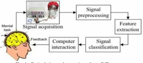
By e xtracting specific co mponents fro m human bra in activity and linking this brain activity to specifica lly developed algorith ms, an interface between a computer and the users’ brain is created. Current BCI designs typically incorporate five ma in stages as shown in Fig. 1. Signals fro m the brain are processed to extract specific features that reflect the user’s intentions. Today there exist various techniques by which to accomplish this [7-12]. The user’s brain is now coupled to a computer or e xte rnal device , which allow co mmunication or controlling devices directly, without imple ment ing any motor action. In this paper, a nonlinear independent component analysis (NICA) e xtract ion method entailing t ime-series EEG signals is proposed. In order to exa mine the performance (i.e., accuracy and transfer rate) imp rovements of the proposed method, a classification using Fisher’s Linear Discriminant Analysis (FLDA) which has been well developed in the field of speech recognition is applied.
The contributions of this study are as follows.
(i) Enhancement and strengthening of art ifacts -contaminated and stochastic EEG signals utilizing the small-a mplitude of the EEG-P300.
(ii) Driving of the trac king error to a s mall value around zero while guaranteeing the closed-loop stability.
(iii) Improve ment of the classification accuracy and transfer rate of a BCI by application of the proposed NICA method, even when subjects are in a fatigued condition. The structure of the paper is as fo llo ws. Sect ion II discusses the EEG data set and its preprocessing. Section III e xp lains feature e xtraction and classificat ion by the NICA method and the FLDA, respectively. Results are discussed in Section IV, and conclusions are drawn in Section V.
Feature Extraction of EEG-P300 Signals Using
Nonlinear Independent Component Analysis
Arjon Turnip dan Demi Soetraprawata
II. DAT A SET AND EEGPREPROCESSING
The acquired signals are preprocessed to reduce externa l noises and detected artifacts. The filtered signals are then sent to the feature ext raction and classification module, respectively. Since the purpose of this chapter is to demonstrate the performance of the co mpared e xt raction method, the present study utilizes the same raw data used in the work of Hoffmann et al., 2008 [13]. A lso, only the data of 8 out of 32 channels (i.e., Fz, Cz, Pz, Oz, P7, P3, P4, and P8) placed at the standard positions described in the 10-20 International System [14] are used, which is claimed to be sufficient, in that a good compro mise between the sufficiency of accuracy and the computational comp le xity in handling mu ltiple channels is achieved.
The EEG signals we re recorded at 2048 Hz samp ling rate. The duration of each image flash (Fig. 2) was 100 ms, fo llo wed by a 300ms blank screen (i.e., the inter-stimu lus interval was 400 ms). One tria l takes about 400 ms; six trials make one segment; about 20~25 segments ma ke one run; six runs make one session and four sessions are designed for individual subject. Therefore, one session involves 810 trials, and the entire data for one subject, therefore, was taken fro m an average of 3240 tria ls. Prior to feature e xtraction, several preprocessing operations including filtering and down-sampling we re carried out. To filter the data, a 6th-order band-pass filter (BPF) with cutoff frequencies of 1 Hz (i.e ., to re move the trend from low frequency bands) and 12 H z (i.e., to re move unimportant informat ion in h igh frequency bands) was used.
It is difficult to co mpare the performances of the BCI systems, because the pertinent studies present the results in diffe rent ways. However, in the present study, the comparison was made based on the accuracy and the transfer rate. Accuracy is perhaps the most important aspect in any BCI. Besides accuracy, the transfer rate is also very important. The speed of a particular BCI is affected by the tria l length, that is, the time needed for one selection. This time should be shortened in order to enhance a BCI’s effectiveness in commun ication. The bit rate (bits/trial) of each selection can then be e xpressed as [15, 16].
1 1 log ) 1 ( ) ( log ) (
log2 2 2
N P P
P P N
b , (1)
where N is a number of possible selections of the target and P
denotes the probability that the desired choice is actually selected. The transfer rate (bits per minute) is equal to b
mu ltip lied by the average speed of selection S (trial per minute, which is equal to the reciprocal of the average time required for one selection). Therefore , based on the data sets information, the desired output signal is developed.
III. FEAT URE EXT RACT ION AND CLASSIFICAT ION
A. Nonlinear Independent Component Analysis
The goal of feature e xtraction is to find data representations that can be used to simplify the subsequent brain pattern classification or detection. The e xtracted signals should encode the commands made by the subject but should not contain noises or other interfering patterns (or at least should reduce their level) that can impede c lassification or increase the difficulty of analy zing EEG signals. Fo r this reason, it is necessary to design a specific e xt raction method that can reduce such artifacts in EEG records. Thus, the compared e xtractor are given to help the user for further research.
The M nonlinear mixed signals x1,,xM are re lated to N
independent source signals s1,,sN through:
) , , (
) , , (
) , , (
1 1 2 2
1 1 1
N M
M
N N
s s f x
s s f x
s s f x
, (2)
which can be written in general form of
) (s f
x (3)
where x is the observed M-dimensional data (mixture) vector, f
is an unknown rea l-va lued M-co mponent mixing function, and
s is an N-vector whose elements are the N unknown independent components. Assume now for simp licity that the number of independent components N equals the number of mixtu res M. The general nonlinear ICA proble m then consists
of finding a mapping h:NN that gives components . To reconstruct the original signals, another nonlinear transformation is applied to x1,,xN to get y1,,yN through:
) , , (
) , , (
) , , (
1 1 2 2
1 1 1
N N
N
N N
x x h y
x x h y
x x h y
, (4)
or equivalently to
) (x h
that are statistically independent. A fundamental characteristic of the nonlinear ICA proble m is that in the general case, solutions always e xist, and they are highly non -unique. One reason for this is that if x and y are two independent random variables, any of their functions f(x) and g(y) are also
independent. An even more serious proble m is that in the nonlinear case, x and y can be mixed and still statistically independent. In the respective nonlinear ICA proble m, one should find the original source signals s that has generated the observed data. An important special case of the general nonlinear mixing model (5) consists of so-called post-nonlinear mixtures. There each mixture has the form
n
j j ij i
i f a s
x
1
, i1,,n (6)
Thus the sources sj,j1,,n are first mixed linearly according to the following basic ICA model
n
j j ja
s As x
1
, (7)
but after that a nonlinear function fi is applied to them to get the final observations xi. The goal is to find a specific model that exp lains how the observations were generated. In this study, the amounts to estimating both the source signals s and the unknown mixing mapping f() that have generated the
observed data x through the general mapping (3).
Given m independent variables y(y1,,ym) and a variable x, a new variable ym1g(y,x) is constructed so that the set y1,,ym1 is mutually independent. The construction is defined recursively as fo llo ws. Assume that we have a lready independent random variables y1,,ym which are jo intly uniformly distributed in [0,1]m. Here it is not a restrict ion to
assume that the distributions of the yi are uniform, since this follows directly fro m the recursion, as will be seen below; for a single variable, uniformity can be attained by the probability integral transformation. Denote by x any random variable, and by a1,,am,b some nonrandom scalars. Define
) , , (
, , ,
, , | ;
, , ,
1 1 ,
1 1 ,
1
m y
b
m x
y
m m x
y m
a a p
d a a p
a y a y b x P p b a a g
(8)
where py() and py,x() are the margina l probability densities of y and (y,x) , respectively, and P
| denotes theconditional probability. The py,x in the argu ment of g is to re mind that g depends on the joint probability d istribution of y
and x. For m0, g is simp ly the cu mu lative d istribution
function of x. Now, g as defined above gives a nonlinear decomposition.
A separation method for the post-nonlinear mixtu res (5) should generally consist of two subsequent parts or stages: a nonlinear stage, which should cancel the nonlinear distortions
n i
fi, 1,, . This part consists of nonlinear functions
u
gi i, . The para meters i of each nonlinearity gi are adjusted so that cancellation is achieved. A linear stage that separates the approximate ly linear mixtures v obtained after the nonlinear stage. This is done as usual by learning a nxn
separating matrix B for wh ich the components of the output vector yBv of the separating system are statistically
independent.
Taleb and Jutten [17] use the mutual informat ion I(y)
between the components y1,,yn of the output vector as the cost function and independence criterion in both stages. For the linear part, minimizat ion of the mutual information leads to the familiar Bell-Sejnowski algorithm [18]
1)
(
E xT BT
B y
I
, (9)
where co mponents i of the vector
are score functions of the components yi of the output vectory
:) (
) ( ) ( log )
(
'
u p
u p u p du
d u
i i i
i
. (10)
Here pi(u) is the probability density function of yi and
) (
'
u
pi its derivative. For the nonlinear stage, one can derive the gradient learning rule [17]
n i
k k k k ik i i
k k k k
k
x g b y E
x g E y I
1 '
) , ( ) (
) , ( log )
(
. (11)
Here xk is the kth component of the input vector, bik is the
ele ment ik of the matrix B, and gk' is the derivative of the kth nonlinear function gk. The exact co mputation algorithm
depends naturally on the specific para metric form of the chosen nonlinear mapping gk(k,xk). In [17], mu ltilayer perceptron network (M LPN) is used for modeling the functions
n k
x
gk(k, k), 1,, .
n
i
n
k j ji
ki n
k j ij
ik
g g
g g n
n PI
1 1 1
1 max
1 max
1 1
(12)
where G is the global transformation matrix fro m s to y, gij is
the (i,j) -ele ment of the g lobal system matrix G=HW and ma xj gijrepresents the ma ximu m value a mong the ele ments in the ith
row vector of G, ma xjgij does the ma ximu m value a mong the
ele ments in the ith co lu mn vector of G. When the perfect separation is achieved, the performance inde x is zero. In practice, the va lues of performance inde x around 10-2 gives quite a good performance.
B. Fisher’s Linear Discriminant Analysis
The goal in Fisher’s linear discriminant analysis (FLDA) is to compute a discriminant vector that separates two or more classes as well as possible. Here, we consider only the two-class case. We are given a set of input vectors
N
i
xiD, 1,, and corresponding class -labels
1,1
i
y Denoting by N1 the number of tra ining e xa mples for which yi =1, by C1 the set of ind ices i for wh ich yi = 1, and
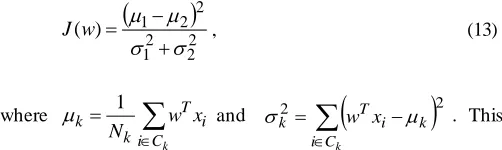
using analogous definitions for N2, C2, the objective function for computing a discriminant vector w[21]
2 2 2 1
2 2 1
) (
w
J , (13)
where
k
C i
i T k
k w x
N 1
and 2
2
k C i
k i T
k w x
. This
means that one is searching for discriminant zectors that result in a large distance between the projected means and small variance around the projected means (sma ll within -c lass variance). To co mpute directly the optima l discriminant vector for a train ing data set, matrix equations for the quantities
22
1
and 12 22 can be used. First, the class means of
k
m is defined
k C i
i k
k x
N
m 1 . (14)
Now we can define the between-class scatter matrix SB and the within-class scatter matrix SW.
Tm m m
m1 2 1 2
B
S , (15)
k C i
T k i k i k
m x m x
2
1 W
S . (16)
With the help of these two matrices the objective function for FLDA can be written as a Rayleigh quotient.
w w
w w w J
T T
W B
S S )
( (17)
By computing the derivative of J and setting it to zero, one can show that the optimal solution for w satisfies the following equation:
1 2
1 W
S m m
w . (18)
A potential proble m in FLDA is that the within -class scatter matrix SW can become singular, and the inverse of SW can become ill-defined. In particular, this happens when the number of features D beco mes larger than the number of training e xa mples N. A simp le solution for this proble m is to replace the inverse SW1 by the Moore–Penrose pseudo-inverse
W
S [22]. The output of FLDA g iven an input vector xˆ is
simp ly the product wTxˆ . In the P300-based BCI described in
the present study, the output of FLDA was summed over t ria ls and the image corresponding to the ma ximu m of the summed output values was then selected.
IV. RESULT S AND DISCUSSION
In this paper, a new method using nonlinear independent component analysis for e xtra xt ion of EEG-P300 signals is proposed. The EEG signals were first preprocessed using a sixth-order band-pass filter (BPF) with cut-off frequencies of 1 Hz and 12 Hz, respectively, see Fig. 3. It can be seen that the signals were corrupted by noises. The feature e xt raction of the pre-processed signals of the eight electrodes (Fz, Cz, Pz, Oz, P7, P3, P4, and P8) can be co mpared with the e xtraction using NICA method in Fig. 4. The features were e xtracted every 400 ms interval (one trial) for about 120 target tria ls. Fro m the results in Fig. 4, a lthough the signals were still corrupted by noises (i.e., ma rked with h igh a mp litude of non-target at some trials), the behaviors of the e xtracted signals clearly represent the EEG-based P300 evoked potentials (i.e., ma rked with higher amplitude of the target).
.
0 5 10 15 20 25 30 35 40 45 50
0 Fz Cz Pz Oz P7 P3 P4 P8
C
ha
nn
el
Time [s] Stimulus
.
0 5 10 15 20 25 30 35 40 45 50
Fz Cz Pz Oz P7 P3 P4 P8
C
ha
nn
el
Time [s]
Target and Non Target Target and Non Target
Stimulus
Fig. 4. Feature extraction using NICA algorithm.
Plots showing the tracking error with and without application of the NICA approach are drawn in Fig. 5. The curves indicate that with the NICA method, a leve l of accuracy is attained after about 240 iterations. Contrastingly, when the p roposed feature e xtraction method is not used, the same level of accuracy is attained only after 1800 iterat ions . These results show clearly that introduction of the NICA methods accelerates the training processes. The tracking error converges to a small va lue around zero, and the closed-loop stability is guaranteed. Furthermore, with the NICA algorithm, the convergence is faster.
Fig. 5. Network’s performance according to mean square errors (ie., blue and red with and without NICA, respectively).
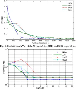
In the present study, the performance of the proposed e xtraction method is tested using a FLDA classifie r. In order to cope with nonlinearly separable problems, additional layers of neurons placed between the input layer and the output neuron are needed, leading to the multilayer perceptron architecture. At the outset, the structure of the network is chosen, after wh ich the validation pattern appears in the graph window, and the network in itia lizat ion values are introduced. Each subsequent layer has a we ight coming fro m the previous layer. Performance is measured according to the specified performance function such as iteration speed and signal noise to ratio (SNR) criteria [23, 24]. The robustness of the proposed e xtraction algorith m was evaluated by comparing its separation performance with well-known algorith ms (i.e ., adaptive autoregressive model (AAR), jo int appro ximate diagonalization of eigen matrices (JADE), and second-order blind identificat ion (SOBI)) as shown in Fig. 6. Until all iteration, the NICA a lgorith m perform better performance inde x. Th is values indicate that the output of the proposed method gives better results for short training time . Fig. 7 shows
0 500 1000 1500 2000 2500 3000 3500 4000 4500 5000 0
0.1 0.2 0.3 0.4 0.5 0.6 0.7
Number of iterations k
PI
(k
) [
dB
]
NICA AAR JADE SOBI
Fig. 6. Evolutions of PI(k) of the NICA, AAR, JADE, and SOBI algorithms.
-2 0 2 4 6 8 10 12 14 16 18
-102
-101
-100
SNR [dB]
Pe
rfo
rma
nc
e
In
de
x
NICA AAR JADE SOBI
Fig. 7. Comparison of performance index of the NICA, AAR, JADE, and SOBI algorithms as a function of signal to noise ratio (SNR).
typical performances of the comparat ive algorith ms discussed in this paper. At high SNR, a ll tested algorithms perform very well. At low SNR, one can observe that the NICA method gives better performance than the other algorith ms in most SNR ranges. In 0 - 4dB range SOBI is worse than the others.
The data sets for subject 5 were not included in the simu lation since the subject misunders tood the instructions given before the experiment. Co mparative plots of the classification accuracies and transfer rates (obtained with the others well known e xt raction method and averaged over four sessions based on the eight electrode configuration s) for the disable- (S1 - S4) and able-bodied subjects (S6 - S9) are depicted in Fig. 8 and Fig. 9, respectively. All of the subjects (using NICA e xt raction method), e xcept for subject 9, achieved an average classification accuracy of 100% after five blocks of stimulus presentations were averaged (i.e ., around 14 s). The reason for the poorer performance of subject 9 might be fat igue. Moreover, the performance of the proposed extraction method also can be seen in Fig. 10 (i.e., average of the disable subjects ), Fig. 11 (i.e., average of the able-body subject), and Fig. 12 (i.e., average of all subjects). Those figures indicated that the proposed extraction method were superior compared to others e xtraction method. Shown alongside the classification accuracies for a ll o f the subjects, in Table I, are the corresponding 93%, 94%, 92%, and 96% confidence intervals corresponding to extraction methods using SOBI, JADE, AAR, and NICA, respectively. Those values indicated that the results achieved through NICA method we re highly superior
0 500 1000 1500 2000 2500 3000 0
100 200 300 400 500 600
Epoch
Su
m
-S
qu
ar
ed
E
rro
r
compared to others method. If we analy ze the results for accuracy (see Table I), the disabled subjects obtained slightly better performance both with and without the proposed feature e xtraction method e xcept with SOBI e xt raction. These results reflect the fact that the brain signals of the disabled subjects were less noisy and more homogeneous than those of the able-bodied subjects.
The transfer rates corresponding to the FLDA classification accuracies for the eight-electrode configuration were tested. The results showed that significant imp rovements in both classification accuracy and average transfer rate were obtained. The ma ximu m average transfer rates, the mean t ransfer rates, and the standard deviations for all co mbinations of the feature e xtraction algorithm are listed in Table II. These results show that the maximu m average transfer rates for all of the subjects
0 5 10 15 20 25 30 35 40 45 50 0 10 20 30 40 50 60 70 80 90 100 A c c u ra c y ( % ) Time (s)
0 5 10 15 20 25 30 35 40 45 50 0 5 10 15 20 25 30 35 40 45 50 0 5 10 15 20 25 30 35 40 45 50 0 5 10 15 20 25 30 35 40 45 50 Subject 1 Accuracy
Transfer rate
0 5 10 15 20 25 30 35 40 45 50 0 10 20 30 40 50 60 70 80 90 100
0 5 10 15 20 25 30 35 40 45 500
5 10 15 20 25 30 35 40 45 50
0 5 10 15 20 25 30 35 40 45 500
5 10 15 20 25 30 35 40 45 50
0 5 10 15 20 25 30 35 40 45 500
5 10 15 20 25 30 35 40 45 50
0 5 10 15 20 25 30 35 40 45 500
5 10 15 20 25 30 35 40 45 50 Tr a n s fe r ra te ( b it s /m in ) Subject 2
0 5 10 15 20 25 30 35 40 45 50
0 10 20 30 40 50 60 70 80 90 100 A c c u ra c y ( % ) Time (s)
0 5 10 15 20 25 30 35 40 45 500
5 10 15 20 25 30 35 40 45 50
0 5 10 15 20 25 30 35 40 45 500
5 10 15 20 25 30 35 40 45 50
0 5 10 15 20 25 30 35 40 45 500
5 10 15 20 25 30 35 40 45 50
0 5 10 15 20 25 30 35 40 45 500
5 10 15 20 25 30 35 40 45 50 Subject 3
0 5 10 15 20 25 30 35 40 45 50
0 10 20 30 40 50 60 70 80 90 100 Time (s)
0 5 10 15 20 25 30 35 40 45 500
5 10 15 20 25 30 35 40 45 50
0 5 10 15 20 25 30 35 40 45 500
5 10 15 20 25 30 35 40 45 50
0 5 10 15 20 25 30 35 40 45 500
5 10 15 20 25 30 35 40 45 50
0 5 10 15 20 25 30 35 40 45 500
5 10 15 20 25 30 35 40 45 50 Tr a n s fe r ra te ( b it s /m in ) NICA AAR SOBI JADE Subject 4 Accuracy Transfer rate
Fig. 8. Comparison of classification accuracy and transfer rate plots (averaged over four sessions based on eight electrode configurations) for disabled subjects
(subjects 1- 4).
0 5 10 15 20 25 30 35 40 45 50 0 10 20 30 40 50 60 70 80 90 100 A c c u ra c y ( % )
0 5 10 15 20 25 30 35 40 45 50 0 5 10 15 20 25 30 35 40 45 50 0 5 10 15 20 25 30 35 40 45 50 0 5 10 15 20 25 30 35 40 45 50 Subject 6
0 5 10 15 20 25 30 35 40 45 50 0 10 20 30 40 50 60 70 80 90 100
0 5 10 15 20 25 30 35 40 45 500
5 10 15 20 25 30 35 40 45 50
0 5 10 15 20 25 30 35 40 45 500
5 10 15 20 25 30 35 40 45 50
0 5 10 15 20 25 30 35 40 45 500
5 10 15 20 25 30 35 40 45 50
0 5 10 15 20 25 30 35 40 45 500
5 10 15 20 25 30 35 40 45 50 Tr a n s fe r ra te ( b it s /m in ) Subject 7
0 5 10 15 20 25 30 35 40 45 50 0 10 20 30 40 50 60 70 80 90 100 A c c u ra c y ( % ) Time (s)
0 5 10 15 20 25 30 35 40 45 50 0 5 10 15 20 25 30 35 40 45 50 0 5 10 15 20 25 30 35 40 45 50 0 5 10 15 20 25 30 35 40 45 50 Subject 8
0 5 10 15 20 25 30 35 40 45 50 0 10 20 30 40 50 60 70 80 90 100 Time (s)
0 5 10 15 20 25 30 35 40 45 500
5 10 15 20 25 30 35 40 45 50
0 5 10 15 20 25 30 35 40 45 500
5 10 15 20 25 30 35 40 45 50
0 5 10 15 20 25 30 35 40 45 500
5 10 15 20 25 30 35 40 45 50
0 5 10 15 20 25 30 35 40 45 500
5 10 15 20 25 30 35 40 45 50 Tr a n s fe r ra te ( b it s /m in ) NICA AAR SOBI JADE Subject 9 Accuracy Transfer rate
Fig. 9. Comparison of classification accuracy and transfer rate plots (averaged over four sessions based on eight electrode configuration s) for able-bodied
subjects (subject s 6- 9).
0 5 10 15 20 25 30 35 40 45 50
0 10 20 30 40 50 60 70 80 90 100 A c c u ra c y ( % ) Time (s)
0 5 10 15 20 25 30 35 40 45 50
0 5 10 15 20 25 30 35 40 45 50
0 5 10 15 20 25 30 35 40 45 50
0 5 10 15 20 25 30 35 40 45 50
Tr a n s fe r ra te ( b it s /m in ) NICA AAR SOBI JADE Averages of subject 1-4 Accuracy Transfer rate
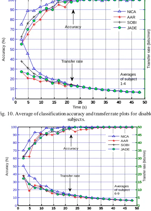
Fig. 10. Average of classification accuracy and transfer rate plots for disabled subjects.
0 5 10 15 20 25 30 35 40 45 50
0 10 20 30 40 50 60 70 80 90 100 A cc ur ac y (% ) Time (s)
0 5 10 15 20 25 30 35 40 45 50
0 5 10 15 20 25 30 35 40 45 500
5 10 15 20 25 30 35 40 45 50
0 5 10 15 20 25 30 35 40 45 500
5 10 15 20 25 30 35 40 45 50
0 5 10 15 20 25 30 35 40 45 500
5 10 15 20 25 30 35 40 45 50 Tr an sf er r at e (b its /m in ) NICA AAR SOBI JADE Averages of subject 6-9 Accuracy Transfer rate
Fig. 11. Average of classification accuracy and transfer rate plots for disabled subjects.
0 5 10 15 20 25 30 35 40 45 50
0 10 20 30 40 50 60 70 80 90 100 A cc ur ac y (% ) Time (s)
0 5 10 15 20 25 30 35 40 45 50
0 5 10 15 20 25 30 35 40 45 500
5 10 15 20 25 30 35 40 45 50
0 5 10 15 20 25 30 35 40 45 500
5 10 15 20 25 30 35 40 45 50
0 5 10 15 20 25 30 35 40 45 500
5 10 15 20 25 30 35 40 45 50 Tr an sf er r at e (b its /m in ) NICA AAR SOBI JADE Averages of all subject Accuracy Transfer rate
Fig. 12. Average of classification accuracy and transfer rate plots for all subjects.
confirmed the BCI-applicab ility of the proposed extraction method. By contrast, the classification accuracies and transfer rates obtained using the well known e xt raction methods separately were found to be only margina lly superior to mere chance, indicating the inadequacy of those methods for BCI applications.
One negative characteristic of P300 detection is that the amp litude of the waveform requires the averaging of mult iple recordings to isolate a signal. In order to streamline the averaging process, the proposed feature e xtraction modules were applied to segments of EEG signals (EEG t ria ls). These modules are integral to the c lassification accuracy and t ransfer rate of the mental act ivities. A factor re lating to the attain ment of good classification accuracy and transfer rates for disabled subjects, both in commun ication systems and BCI systems, is the sequence of a given stimulus. When applying the proposed method to e xt ract EEG s ignal features, it was found that any two sequential ta rget stimuli e xc ite just one P300 co mponent peak, and are e xt racted in that form. Ho wever, in order that EEG signals be classified with 100% accuracy, such stimuli must e xcite two peaks of a mp litude. Therefo re, in order to obtain a good classification accuracy and transfer rate, the given stimulus must be inputted randomly with a constraint. In other words, two targets should not be flashed sequentially.
TABLE I
AVERAGE CLASSIFICATION ACCURACY (%)
Subject SOBI JADE AAR NICA
S1 94.00 93.00 88.75 94.50
S2 92.25 94.50 90.00 97.30
S3 94.00 95.50 95.00 97.70
S4 93.00 94.25 94.50 97.25
S6 90.50 91.85 90.55 96.50
S7 94.75 94.00 93.20 96.25
S8 94.75 96.00 94.50 96.35
S9 93.70 92.95 90.00 97.50
Average
(S1–S4) 93.30.8 94.31.0 92.13.1
96.71.4
Average
(S6-S9) 93.42.0 93.71.7 91.12.1
96.60.5
Average
(all) 93.41.4 94.01.3 92.12.4
96.61.0
TABLE II
AVERAGE TRANSFER RATE (%)
Subject SOBI JADE AAR NICA
S1 17.13 17.13 8.13 17.13
S2 12.58 17.48 10.60 34.96
S3 17.48 25.17 25.17 34.96
S4 11.77 17.13 17.48 34.96
S6 10.60 17.13 20.95 25.17
S7 17.13 17.13 17.13 25.17
S8 25.17 25.17 20.95 19.34
S9 17.13 17.13 17.13 34.96
Average
(S1–S4) 14.7 2.9 19.2 3.9 15.37.6 30.5 8.9 Average
(S6-S9) 17.5 5.9 19.1 4.0 19.02.2 26.2 6.4 Average
(all) 16.1 4.6 19.1 3.6 17.25.5 28.3 7.5
V. CONCLUSIONS
The results presented in this study show that, compared with the well known e xt raction algorith ms, a better e xtract ion result can be obtained when using the NICA a lgorith m (i.e., faster training and higher SNR) for single -trial ERPs based on the P300 co mponent fro m specific bra in regions . With NICA e xtraction, the data indicate that a P300-based BCI system can communicate at the rate around 34.96 b its/min for the disable- and able-bodied subjects . The average of 100% classification accuracy is achieved after four blocks (average) for disabled subjects and after five blocks (average) for able -bodied subjects. To improve our results, we are currently investigating the effect of averaging the output of the classifier over the consecutive windows as well as the effects of other preprocessing methods in artifact-effect reduction.
A
CKNOWLEDGMENTThis research was supported by the tematic progra m (No. 3425.001.013) through the Bandung Technical Management Unit for Instrumentation Development (Deputy for Scientific Services) funded by Indonesian Institute of Sciences, Indonesia.
REFERENCES
[1] E. R. Kandel, J. H. Schwartz, and T. M. Jessel, editors, The Principles of
Neural Science, Prentice Hall, 3rd edition, 1991.
[2] S. Sutton, M. Braren, E. R. John, and J. Zubin, “Evoked potential
correlates of stimulus uncertainty,” Science, vol.150, no. 700, pp.
1187-1188, 1965.
[3] E. Donchin, K. M. Spencer, and R. Wijesinghe, “The mental prosthesis:
Assessing the speed of a P300-based brain–computer interface,” IEEE
Trans. Rehabil. Eng., vol. 8, no. 2, pp. 174-179, 2000.
[4] G. Pfurtscheller, C. Neuper, A. Schlogl, and K. Lugger, “ Separability of
EEG signals recorded during right and left motor imagery using adaptive
autoregressive parameters,” IEEE Trans. Rehabil. Eng., vol. 6, no. 3, pp.
316-325, 1998.
[5] F. Aloise, F. Schettini, P. Arico, F. Leotta, S. Salinari, D. Mattia, F.
Babiloni, F. Cincotti, “P300-based brain-computer interface for
environmental control: An asynchronous approach,” Journal of Neural
Engineering, vol. 8, no. 2, 025025, 2011.
[6] A. Belitski, J. Farquhar, and P. Desain, “P300 audio-visual speller,”
Journal of Neural Engineering, vol. 8, no. 2, 025022, 2011.
[7] M. Arnold, U. Moller, and H. Witte, “Nonlinear time-series modeling by
means of self-exciting threshold AR models,” Theory in Biosciences, vol.
118, no. 3-4, pp. 261-266, 1999.
[8] H. Cecotti and A. Graser, “ Convolutional neural networks for P300
detection with application to brain-computer interfaces,” IEEE Trans.
Pattern Anal. Mach. Intell., vol. 33, no. 3, pp. 433-445, 2011.
[9] Z.-G. Che, T.-A. Chiang, and Z.-H. Che, “ Feed-forward neural networks
training: A comparison between genetic algorithm and back-propagation
learning algorithm,” Int. J. Innov. Comp. Inf. Control, vol. 7, no. 10, pp.
5839-5851, 2011.
[10] J. Escudero, R. Hornero, D. Abasolo, A. Fernandez, “Quantitative
evaluation of artifact removal in real magnetoencephalogram signals with
blind source separation,” Annals of Biom edical Engineering, vol. 39, no.
8, pp. 2274-2286, 2011.
[11] A. T urnip and K.-S. Hong, “ Classifying mental activities from EEG-P300
signals using adaptive neural network,” Int. J. Innov. Comp. Inf. Control,
vol. 8, no. 9, pp. , 2012.
[12] A. T urnip, K.-S. Hong, and M.-Y. Jeong, “ Real-time feature extraction of
P300 component using adaptive nonlinear principal component analysis,”
[13] U. Hoffmann, J.-M. Vesin, and T. Ebrahimi. An efficient P300-based
brain–computer interface for disabled subjects. Journal of Neuroscience
Methods, vol. 167, no. 1, pp. 115-125, 2008.
[14] H. H. Jasper, “ Report of the committee on methods of clinical
examination in electroencephalography,” Electroenceph. Clin.
Neurophysiol., vol. 10, pp. 370-375, 1958.
[15] E. W. Sellers, D. J. Krusienski, D. J. McFarland, T. M. Vaughan, and J. R.
Wolpaw, “A P300 event-related potential brain-computer interface (BCI): The effects of matrix size and inter stimulus interval on performance,”
Biological Psychology, vol. 73, no. 3, pp. 242-252, 2006.
[16] J. R. Wolpaw, H. Ramoser, D. J. McFarland, and G. Pfurtscheller,
“EEG-Based Communication: Improved Accuracy by Response
Verification,” IEEE Trans. On Rehab Eng., vol. 6, no. 3, pp. 326-333,
Sept 1998.
[17] A. J. Bell and T. J. Sejnowski, “An informationmaximization approach to
blind separation and blind deconvolution,” Neural Computation, vol. 7,
pp. 1129–1159, 1995.
[18] A. Taleb and C. Jutten. Source separation in post-nonlinear mixtures.
IEEE Trans. On Signal Processing, 47(10):2807–2820, 1999.
[19] A. Hyvarinen, J. Karhunen ,E. Oja. Independent component analysis.
John Wiley & Sons,Inc, ISBN 0-471-40540-X, 2001.
[20] A. Cichocki and S. Amari, Adaptive blind signal and image processing,
New York, USA: Wiley, 2002, pp. 161-162.
[21] M. Kaper, P. Meinicke, U. Grosskathoefer, T . Lingner, R.
Ritter, ”Support vector machines for the P300 speller paradigm,” IEEE
Trans. Biom ed. Eng.,vol. 51, no. 6, pp. 1073–1079, 2004.
[22] Q. Tian, Y. Fainman, S. H. Lee, “ Comparison of statistical
pattern-recognition algorithms for hybrid processing. II.
Eigenvector-based algorithm, “J. Opt. Soc. Am . A., vol. 5, no. 10 pp.
1670–82, 1988.
[23] S. Choi and A. Cichocki, “Blind separation of nonstationary sources in
noisy mixtures,” Electronics Letters, vol. 37, no. 1, pp. 61-62, 2001.
[24] S. Choi, A. Cichocki, and A. Belouchrani. Second order nonstationary
![Fig. 2. The display used for evoking EEG-P300 signals [13].](https://thumb-us.123doks.com/thumbv2/123dok_us/1372907.1647353/2.612.69.292.537.727/fig-display-used-evoking-eeg-p-signals.webp)