Abstract—Developing a precise and accurate model of gold price is critical to manage assets because of its unique features. In this paper, artificial neural network (ANN) model have been used for modeling the gold price, and compared with the traditional statistical model of ARIMA (autoregressive integrated moving average). The three performance measures, the coefficient of determination (R2), root mean squared error (RMSE), mean absolute error (MAE), are utilized to evaluate the performances of different models developed. The results show that the ANN model outperforms ARIMA model, in terms of different performance criteria during the training and validation phases.
Index Terms—ANN, gold price, forecasting, ARIMA.
I. INTRODUCTION
Gold price plays a significant role in economical and monetary systems. The price of gold and other assets are often closely correlated [1]. For example, the link between gold and equities is usually negative, as investors typically transfer money from gold into the safe haven of equities during times of boom and vice versa during times of crisis. Whereas, the link between gold and oil is typically positive and a tension can lift both the price of oil and gold.
Accurate forecasting of gold price helps to foresee the circumstances of trends in the future. This provides the useful information for stakeholder to fulfill the essential actions in order to prevent or mitigate risks, which may lead to financial losses or even bankruptcy.
Traditional mathematical models such as Autoregressive Integrated Moving Average [2], jump and dip diffusion [3], and the multi linear regression [4]-[7] models have been used for gold price forecasting. As well as, artificial intelligence models such as artificial neural networks (ANN) have been developed as a non-linear tool for gold price forecasting [2], [5], [8].
These studies document the need for a better management of gold selling and investing to reduce risk value. An accurate gold price forecasting model is needed to show the trend of price changes in the futures to carry out appropriate exchanges. Furthermore, it is very difficult to earn a powerful function using traditional mathematical model [5], and these models are principally based on some strong assumptions and prior knowledge of input data statistical distributions.
The main aim of this paper is to analyze the capability of an ANN in modeling gold price changes and to evaluate its
Manuscript received November 9, 2013; revised January 22, 2014. Hossein Mombeini is with the Faculty of finance, Islamic Azad University, Dubai branch, Dubai, UAE (e-mail: h.mombeini@yahoo.com).
Abdolreza Yazdani-Chamzini is with the South Tehran Branch, Islamic Azad University, Tehran, Iran (e-mail: abdalrezaych@gmail.com).
performance in comparison with other traditional time series modeling techniques such as ARIMA. Finally, the best fit model is identified according to the performance criteria including coefficient of determination (R2), mean absolute error (MAE), and root mean square error (RMSE).
The rest of the paper is organized as follows: Section II summarizes artificial neural networks. Section III describes the ARIMA model, including the determination of the orders of ARMA model. Section IV presents the gold price modeling by ANN and ARIMA models. Section V analyzes the performance of the models, including its comparison with other and discusses several practical issues involved in its deployment. Sensitivity analysis is presented in Section VI presents. Finally, the conclusions of the present study are discussed in Section VII.
II. ARTIFICIAL NEURAL NETWORKS (ANN)
ANN technique has emerged as a powerful modeling tool which can be applied for many scientific and/or engineering applications, such as: pattern reorganization, classification, data processing, and process control. ANN technique has some unique futures which distinguish them from other data processing systems include ability to work successfully even when they are party damaged, parallel processing, ability to make generalization, and little susceptibility to errors in data sets [9]. An artificial neural network simulates the human brain mechanism to implement computing behavior [10].
ANN is developed based on biological neural networks, which neurons are the basic building blocks ones. An artificial neuron is a model of a biological neuron. An artificial neuron receives signals from other neurons, gathers these signals, and when fired, transmits a signal to all connected neurons [11]. An artificial neuron model is depicted in Fig. 1.
1
n
i ij i j i
y f w x
(1)f is generally linear, step, threshold, logarithmic sigmoid (logsig), hyperbolic tangent sigmoid (tansig) functions.
Fig. 1. Artificial neuron model.
Modeling Gold Price via Artificial Neural Network
Hossein Mombeini and Abdolreza Yazdani-Chamzini
As seen in Fig. 1, xi(i= 1, 2, ..., n) is the input signal of n
other neurons to a neuron j; is the connection weight between the ithneuron and the neuron j; is the activation threshold of
the neuron j; fis the transfer function, and yjis the output of
A neural network contains of three layers, including one input layer, several middle layers (hidden layers) and one output layer. It should be noted that there is no theoretical limit on the number of hidden layers but typically there is just one or two [12]. Fig. 2 depicts an artificial neural network architecture employed in this study.
Fig. 2. A typical artificial neural network architecture.
In this study a multi-layer feed-forward perceptron (MLP) with a back propagation learning algorithm is employed to model gold price. During the modeling stage, coefficients are adjusted through comparing the model outputs with actual outputs. A five-step procedure can be described to present the learning process of an ANN as follows:
Input–output vectors are randomly selected as training datasets,
The structure of network is formed,
Network outputs are computed for the selected inputs,
Connection weights are adjusted according to performance measure,
The process of adjusting the weights is continued until performance measures are satisfied.
III. ARIMAMETHOD
Box and Jenkins developed a general forecasting methodology for time series generated by a stationary autoregressive moving-average process [13]. In an autoregressive integrated moving average (ARIMA) model, the future value of a variable is assumed to be a linear function of several past observations and random errors. The term integrated indicates the fact that the model is produced by repeated integrating or summing of the ARMA process [14]. The ARIMA model is employed for applications to nonstationary time series that become stationary after their differencing. The general form of the ARIMA model is given by:
( ) ( ) ( )(1 )d ( )
B x t B B x t
(2)
forecasting. These phases are described in details by Palit and Popovic [14]. In order to determine the order of the ARIMA best model, the autocorrelation function (ACF) and the partial ACF (PACF) of the sample data are employed. In this study, selection technique in conjunction with ACF and PACF for estimating the orders of ARMA model is the Akaike information criterion (AIC). This involves choosing the most suitable lags for the AR and MA components, likewise assigning if the variable requires differencing to convert into a stationary time series.
IV. MODELING OF GOLD PRICE
The information used in this study includes 220 monthly observations of the gold price per ounce against its affecting parameters from April 1990 to July 2008. The gold price changes during this period are depicted in Fig. 3. In order to develop ANN and ARIMA models for the gold price, the available data set, which consists of 220 input vectors and their corresponding output vectors from the historical data of gold price, was separated into training and test sets as depicted in Fig. 4. For achieving the aim, 200 observations (from April 1990 to November 2006) are first applied to formulate the model and the last 20 observations (from December 2006 to July 2008) are used to reflect the performance of the different constructed models. Based on the ARIMA model, the past observations of gold price are used in order to formulate the model, and in order to develop ANN model, the affecting parameters on gold price are extracted as described in the following part.
Fig. 3. Gold price changes (data resource: www.kitco.com).
One of the most important steps in developing a successful forecasting model is the selection of the input variables, which determines the architecture of the model. Based on the „hunches of experts‟, seven input parameters for the gold price forecasting were identified: USD Index (measures the performance of the United States Dollar against the Canadian Dollar), inflation rate (the United States inflation rates), oil price (West Texas Intermediate Crude Oil Prices), interest rate (the United States interest rates), stock market index (Dow Jones Industrial Average), silver price, and world gold production. The data used in this study were downloaded from several sources from the addresses as presented in Table I. As shown in Table I, expect of world gold production, other parameters are monthly. According to the importance of production on the gold price changes, the authors employed the method of Cubic Spline interpolation (see [15]), The structure of ARIMA model is known as ARIMA (p, q,
d), where p stands for the number of autoregressive parameters, q is the number of moving-average parameters, and d is the number of differencing passes.
which is a useful technique to interpolate between known data points due to its stable and smooth characteristics, in order to convert annually data into monthly data. The above mentioned models are established as described in the next section.
ARIMA modal. Using the Eviews package software, the best-fitted model is obtained based on the optimum solution of the parameters (the values of p, d, q) and the residuals (white noise). The best-fitted model is ARIMA (1, 1, 0) as follows:
1
1.873 1.008
t t
y y
(3)
ANN model. According to the concepts of ANNs design and using productive algorithm in MATLAB 7.11 package software in order to obtain the optimum network architecture;
several network architectures are established to compare the ANNs performance. Before constructing the ANN model, all variables were normalized to the interval of 0 and 1 to provide standardization using Eq. (4):
min max min
( ) / ( )
norm
X XX X X
(4) The best fitted network based on the best forecasting accuracy with the test data is contained of seven inputs, twenty four hidden and one output neurons (in abbreviated form, N(7-24-1) ). This confirms that simple network structure that has a small number of hidden nodes often works well in out-of-sample forecasting [16]-[20]. This can be due to the over fitting problem in neural network modeling process that allows the established network to fit the training data well, but poor generalization may happen.
Variable Type of data Maximum Minimum Unit Symbol Resource
Gold price Monthly
1134.72 256.675 $/ounce G www.kitco.com
Silver price Monthly 18.765 3.64 $/ounce S www.kitco.com
USD index Monthly 1.599 0.967 - C research.stlouisfed.org
Oil price Monthly 133.93 11.28 $/barrel O www.economagic.com
Inflation rate Monthly 0.0628 -0.0209 - Inf www.inflationdata.com
www.rateinflation.com
Interest rate Monthly 8.89 2.42 - Int www.econstats.com
stock market index
Monthly 13930 2442.33 $ DJ finance.yahoo.com
www.google.com World gold
production
Annually 216.95 178.195 Ton Pg minerals.usgs.gov
2
2 1
2 1
( )
1
( )
N
i i
i N
i i
i
A P R
A A
(5)2 1( )
N
i i
i A P
RMSE
N
(6)
1
N i i i A P
MAE
N
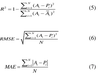
(7) where Pi is predicted values, Ai is observed values,
A
i is the average of observed set, and N is the number of datasets.R2 shows how much of the variability in dependent variable can be explained by independent variable(s). R2 is a positive number that can only take values between zero and
one. A value for R2 close to one shows a good fit of forecasting model and a value close to zero presents a poor fit.
MAE would reflect if the results suffer from a bias between the actual and modeled datasets [21]. RMSE is a used measure in order to calculate the differences between values predicted by a model and the values observed from the thing being modeled. RMSE and MAE are non-negative numbers that for an ideal model can be zero and have no upper bound.
The comparative analysis of testing period performance of the ANN and ARIMA techniques using three global statistical criteria (root mean square error, mean absolute error, and coefficient of determination) has been accomplished and is shown in Table II. According to the table, for ANN and ARIMA models, the RMSE values are 118.04 and 166.87, and the MAE values are 0.102 and 0.144, and R2 values are 0.967 and 0.841, respectively.
For all statistical criteria, the ANN model is better than the ARIMA model, i.e. based on all statistical criteria, the ANN model outperforms the ARIMA model. The results of the study indicate that the forecasting capability of the ARIMA model is poor in comparison with the ANN model in gold price forecasting.
The forecasted value of each model for both validation and training data are plotted in Fig. 4. In addition, the forecasted value of ARIMA and ANN models for test data are plotted in Fig. 5.
TABLE I: STATISTICAL PARAMETERS OFEACH DATA SET
V. PERFORMANCE ASSESSMENT OF THE MODELS
TABLEII:FORECASTING PERFORMANCE INDICES OF MODELS FOR GOLD
PRICE
Model Training Validation
RMSE MAE R2
RMSE MAE R2
ARIMA 14.47 0.025 0.965 166.87 0.144 0.841 ANN 13.21 0.03 0.989 118.04 0.102 0.967
Fig. 4. Actual and forecasted values during training and validation by ARMA and ANN for gold price.
Fig. 5. The variation of the values predicted by ARIMA and ANN models during validation period, from the actual values.
VI. SENSITIVITY ANALYSIS
Sensitivity analysis is a useful tool in order to determine the relationship between the related parameters. In this paper to identify the most sensitive factors affecting gold price cosine amplitude method (CAM) was employed. This approach is a powerful method in order to implement sensitivity analysis [22].
In this method, the degree of sensitivity of each input parameter is assigned by establishing the strength of the relationship (rij) between the gold price and input parameter
under consideration. The larger the value of CAM becomes, the greater is the effect on the gold price, and the sign of every CAM indicates how the input affects the gold price. If the gold price has no relation with the input, then the values are zero, while the input has a positive effect on the gold price when the values are positive and a negative effect on the gold price when the values are negative.
Let n be the number of independent variables represented as an array X={x1, x2, ..., xn}, each of its elements, xi, in the
data array X is itself a vector of length m, and can be expressed as:
1, 2, 3,...,
i i i i im
X x x x x
(8) Thus, each of the data pairs can be thought of as a point in
m dimensional space, where each point requires m coordinates for a complete description. Each element of a relation, rij, results from a pairwise comparison of two data
samples. The strength of the relationship between the data samples, xi and xj, is given by the membership value
expressing that strength:
1
2 2
1 1
, 0 1
m ik jk k
ij ij
m m
ik jk
k k
x x
r r
X X
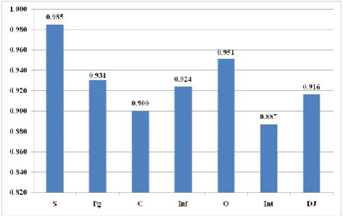
(9)The strengths of relations (rij values) between the gold
price and input parameters are depicted in Fig. 8. As shown in Fig. 8, the most effective parameters on the gold price are silver price and oil price.
Fig. 8. Sensitivity analysis of input parameters.
VII. CONCLUSION
In this study, the performance of different methods for forecasting the gold price changes was investigated. The forecasting methods evaluated include the ANN and ARIMA models. The gold price data from April 1990 to July 2008 were used to develop various models investigated in this study. This comprises 220 input vectors and their corresponding output vectors from the historical data of gold price, which were divided into training and validation sets. Three performance evaluation measures, including MAE, R2, and RMSE, are adopted to analyze the performances of various models developed. The results show that the ANN method is powerful tools to model the gold price and can give better forecasting performance than the ARIMA method. The forecasting results of ANN model during the validation phase outperform the ARIMA model.
REFERENCES
[1] C. Corti and R. Holliday, Gold Science and Applications, Taylor and Francis Group, LLC, 2010.
[2] A. Parisi, F. Parisi, and D. Díaz, “Forecasting gold price changes: Rolling and recursive neural network models,” Journal of Multination Financial Management, vol. 18, pp. 477-487, 2008.
[3] S. Shafiee and E. Topal, “An overview of global gold market and gold price forecasting,” Resources Policy, vol. 35, pp. 178-189, 2010. [4] A. Escribano and C. W. J. Granger, “Investigating the relationship
between gold and silver prices,” Journal of Forecasting, vol. 17, pp. 81-107, 1998.
[5] P. K. Achireko and G. Ansong, “Stochastic model of mineral prices incorporating neural network and regression analysis,” The Institution of Mining and Metallurgy (Sect. A: Min. technol.), vol. 109, pp. 49-54, 2000.
[7] A. A. Kearney and R. E. Lombra, “Gold and platinum: toward solving the price puzzle,” The Quarterly Review of Economics and Finance, vol. 49, pp. 884-892, 2009.
[8] M. C. Lineesh, K. K. Minu, and C. J. John, “Analysis of nonstationary nonlinear economic time series of gold price: a comparative study,”
International Mathematical Forum, vol. 5, pp. 1673-1683, 2010. [9] P. Malinowski and P. Ziembicki, “Analysis of district heating network
monitoring by neural networks classification,” Journal of Civil Engineering and Management, vol. 12, pp. 21-28, 2006.
[10] X. He and S. Xu, Process Neural Networks Theory and Applications, Springer, 2007.
[11] A. P. Engelbrecht, Computational Intelligence: An Introduction, John Wiley & Sons, Ltd., 2002.
[12] S. Sumathi and S. Paneerselvam, Computational Intelligence Paradigms: Theory & Applications using MATLAB, Taylor and Francis Group, LLC, 2010.
[13] P. Box and G. M. Jenkins, “Time series analysis: forecasting and control,” Holden-day Inc, San Francisco, CA, 1976.
[14] A. K. Palit and D. Popovic, “Computational intelligence in time series forecasting: theory and engineering applications,” Springer-Verlag London Limited, 2005.
[15] Ch. W. Ueberhuber, “Numerical computation: methods, software, and analysis,” Springer-Verlag Berlin Heidelberg, vol. 1, 1997.
[16] G. P. Zhang, “Time series forecasting using a hybrid ARIMA and neural network model”, Neurocomputing, vol. 50, pp. 159-175, 2003. [17] M. Khashei, S. R. Hejazi, and M. Bijari, “A new hybrid artificial neural
networks and fuzzy regression model for time series forecasting,”
Fuzzy Sets and Systems, vol. 159, pp. 769-786, 2008.
[18] M. Khashei, M. Bijari, and G. A. R. Ardali, “Improvement of auto-regressive integrated moving average models using fuzzy logic and artificial neural networks (ANNs),” Neurocomputing, vol. 72, pp. 956-967, 2009.
[19] M. Khashei and M. Bijari, “A novel hybridization of artificial neural networks and ARIMA models for time series forecasting,” Applied Soft Computing, vol. 11, pp. 2664-2675, 2011.
[20] P. Areekul, T. Senjyu, H. Toyama, and A. Yona, “A hybrid ARIMA and neural network model for short-term price forecasting in deregulated market,” IEEE Transactions on Power Systems, vol. 25, pp. 524-530, 2010.
[21] R. Khatibi, M. A. Ghorbani, M. H. Kashani, and O. Kisi, “Comparison of three artificial intelligence techniques for discharge routing,”
Journal of Hydrology, vol. 403, pp. 201-212, 2011.
[22] T. J. Ross, Fuzzy Logic with Engineering Applications, Second Edition, John Wiley & Sons Ltd., 2004.
H. Mombeini is a Ph.D student at the Dep. of finance, Dubai branch, Islamic Azad University, Dubai, UAE. He is chief of Samen Sazeh Co. He is the author of more than 10 research papers. His research interests comprise decision making, fuzzy logic, finance, banking, insurance, investment management, forecasting, system analysis, portfolio management, modeling, and optimization.