IJSTE - International Journal of Science Technology & Engineering | Volume 4 | Issue 5 | November 2017 ISSN (online): 2349-784X
Using ARIMA Model to Forecast Sales of an
Automobile Company
Nirbhay Pherwani Vyjayanthi Kamath
UG Student UG Student
Department of Computer Engineering Department of Information Technology Vivekanand Education Society’s Institute of Technology Vivekanand Education Society’s Institute of Technology
Abstract
When it comes to running businesses successfully, sales forecasting is a crucial component to include in the process. In this paper, the aim is to forecast the sales made by an automobile company in a particular city. The data outlines the total sales of the company manufactured cars at the end of the month from 2013 to 2014. Utilizing this data, we fit the Autoregressive Integrated Moving Average (ARIMA) time series with the regression model. Utilizing the Akaike Information Criterion (AIC) and Bayesian Information Criterion (BIC) values, we identify the best fit ARIMA model and use this to obtain the sales forecast for the subsequent year. To successfully build the model we use R Programming.
Keywords: ARIMA, Sales Forecast, Data Analysis, Time Series, Automobile Sales Forecast
________________________________________________________________________________________________________
I. INTRODUCTION
Sales is a rudimentary component which is helpful in guiding the company to cover expenses, decide salaries and wages, in marketing, stocking inventory – the whole deal. Ultimately, sales (and sales forecasting) proves to be an important element when it comes to businesses and companies, be it small or big, old or new. Sales forecasting is beneficial in preparing the company for any unexpected surge/decrease in demand.
The given data is a group of data points obtained at constant time intervals, in a particular city. This is a time series. Being time dependent and possessing some form of seasonality trends (disparity within particular time frames) makes this different than a regular regression, say, a linear one. Hence, a seasonable ARIMA model is the ideal solution. After constructing the ARIMA model we explore it further to find the best fit using certain criteria and optimize it further. Using this finalized model, we obtain the sales forecast for the first half of the following year.
ARIMA Basics
Let’s start with ARMA models – AutoRegressive and Moving Average. These apply exclusively to stationary data. Autoregressive models are built on the concept of current values being dependent on previous values.
Moving Average is built by analysing the averages between several subsets within the entire dataset.
When the data is non-stationary, an extra step is required (differencing) and the two are combined (“integrated”), hence the Integrated component comes into play.
In time series data, there are three particular components to keep in mind: Seasonal: Variations in data WRT calendar cycles.
Cycle: Patters that increase or decrease (not seasonal) Trend: Overall pattern of the time series data
Non seasonal ARIMA models have a specific representation in the form of ARIMA(p,d,q) where p,d,q are parameters: p- the number of time lags.
d- the order of differencing (how many times differencing has been carried out). q- order of the MA model.
II. METHOD
Plot the Data as a Time Series
Fig. 1: A time series plot of the company sales in a city Eliminate Trends and Stabilize Data on Mean (Make it Stationary)
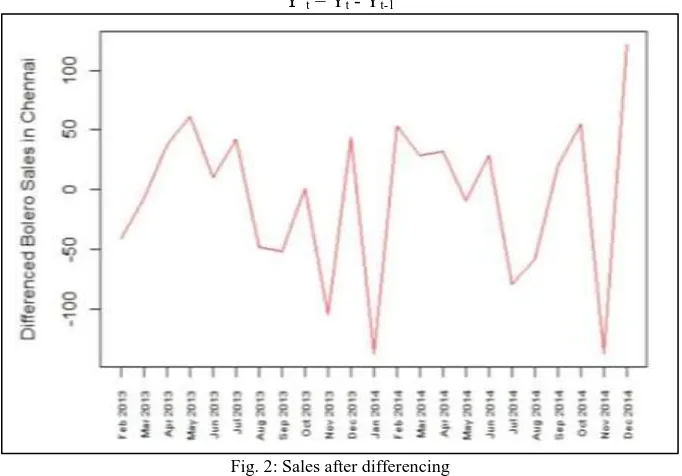
If certain statistical properties are constant over time, the time series is called stationary. This is necessary because if the given data is constant over a particular time frame, the forecast is that much more likely to follow the same consistency. Remove the varying trend in the sales with first order differencing using the formula:
Y’t = Yt - Yt-1
Fig. 2: Sales after differencing
After differencing the data, we find that it isn’t stationary on variance either from Fig 2. The variation within the company sales spans a gradually increasing gap with respect to the time.
Stabilise Data on Variance
Using the below formula, we stabilize the original data over the variance Ynew
Using ARIMA Model to Forecast Sales of an Automobile Company (IJSTE/ Volume 4 / Issue 5 / 015)
Fig. 3: Log transform data to make data stationary on variance Stabilize Data on Variance and ean
After making the data stationary on variance, difference this data to make it stationary on the mean.
Fig. 4: Differenced log transform data to make data stationary on both, mean and variance Plotting ACF & PACF
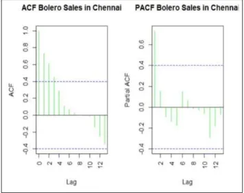
Once the differencing has been carried out and the sales data has been stationarized, we have to figure out the Autoregressive (AR) and Moving Average (MA) terms to eliminate any autocorrelation found in the differenced sales data.
Stationary series have ACF plots that decline to zero quite rapidly.
Autocorrelation Factor (ACF) plot is a bar chart of the correlation coefficients between the time series and their lags.
Fig. 5: ACF and PACF plots Best fit ARIMA Model
The best fit ARIMA model is based on two criterions here:
Akaike Information Criterion - An estimator used to identify the quality of each model relative to others. It is a measure of goodness of fit.
Bayesian Information Criterion – Used in model selection based on a number of parameters The BIC is more consistent compared to the AIC. Generally, the lowest AIC and BIC values are considered
summary(AR) Series: (log10(data)) ARIMA(1,1,0) Coefficients: ar1 -0.5344 s.e. 0.1694
sigma^2 estimated as 0.01112: log likelihood=19.45 AIC=-34.9 AICc=-34.3 BIC=-32.63
Training set error measures:
ME RMSE MAE
Training set -0.0107717 0.1009398 0.07600747 MPE MAPE MASE
Training set -0.5665393 3.229042 0.863658 ACF1
Training set -0.1405711
Using ARIMA Model to Forecast Sales of an Automobile Company (IJSTE/ Volume 4 / Issue 5 / 015)
Forecast Next Year Sales using Best Fit ARIMA
For MA processes, there are spikes in the first one or more lags of ACF. They are also characterized by an exponentially declining PACF, where the number of spikes represents the order of MA. Therefore, here MA = 0.
The readings are all within the threshold values hence we can conclude that there is no more information left to be extracted, thus validating that the ARIMA (1,1,0) is the best fit model for the given car sales data.
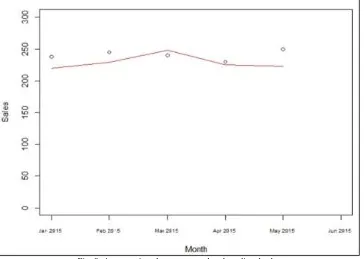
Almost a year later, we received the actual sales figures from the company and found that the predictions were quite close.
Fig. 8: A comparison between actual and predicted sales
In Figure 8, the line represents the actual sales and the plot points represent the predicted sales from the best fit ARIMA model. The percentage error lies in the range between 2% and 12% for the different sales figures.
III. CONCLUSION
In this paper, the problem statement of predicting the sales for an automobile company is considered. It is of interest to note here that, predictions for the next half of the year can be effectively obtained from just two years of past company data. The ARIMA model was used because of its worldwide acceptance and robust features. The auto.arima function provides us with the best fit ARIMA model which is ARIMA (1,1,0). This is validated by analysing the ACF and PACF plots with minimal residuals levels well within the threshold values.
REFERENCES
[1] Time series forecasting using improved ARIMA, IEEE, April 2016
[2] Forecasting Sugarcane Yield of Tamil Nadu Using ARIMA Models, Sugar Tech(Springer), March 2011