O R I G I N A L A R T I C L E
Open Access
Misperceptions of unemployment and
individual labor market outcomes
Ana Rute Cardoso
1*, Annalisa Loviglio
2and Lavinia Piemontese
2*Correspondence: anarute.cardoso@iae.csic.es 1IAE-CSIC, Campus UAB, 08193 Bellaterra, Spain
Full list of author information is available at the end of the article
Abstract
We analyze the impact of misperceptions of the unemployment rate on individual wages, using the European Social Survey. We follow a threefold strategy to tackle potential endogeneity problems, as the model includes the following: controls for worker’s ability, the regional unemployment rate, and country fixed effects. We estimate interval regression models. When subjective perceptions overstate the country unemployment rate, a one percentage point gap between the perceived and the actual rates reduces wages by 0.4 to 0.7 %. We discuss a potential mechanism. A pessimistic view of the labor market leads to concern over own employment prospects, lowering perceived bargaining power and reservation wages. JEL Classification: J31; D80
Keywords: Wage dispersion, Labor market tightness, Perceptions
1 Introduction
The social sciences share an interest in the study of the accuracy of individuals’ percep-tions of issues such as the state of the economy or the prevalence of minority groups in the population. In particular, the search for the factors determining the misperception of unemployment or current inflation has pointed to the relevance of personality traits (Orland 2013), education, cognitive ability, income or wealth, and exposure to media, together with own experience and the situation prevailing in one’s region of residence (see Kunovich 2013; Duffy and Lunn 2009; Blanchflower and Kelly 2008; Conover et al. 1986). In turn, the analysis of the consequences of inaccurate perceptions of the economic situa-tion has concentrated on individuals’ attitudes and behavior. Kunovich (2013) shows that misperception of the unemployment rate has an impact on people’s views on democracy, the role of the State, and labor conflicts. Duffy and Lunn (2009) report that individuals’ misperception of current inflation is negatively related to both consumption and savings intentions.
We contribute to this literature by analyzing the implications of misperceptions of the state of the labor market on actual personal outcomes. Specifically, we evaluate the impact of the misperception of labor market tightness—unemployment rate—on individual wages. Our analysis relies on a direct measure of labor market knowledge imperfections to evaluate its impact on labor market returns.
We exploit information gathered by the European Social Survey (ESS), which included in its 2008 wave a question on the respondents’ degree of information about the job
market. More precisely, individuals were asked for an estimate of the unemployment rate in their country. We take the deviation between their answers and the actual unemploy-ment rate in the country as the degree of misperception of the job market situation. This index is used to explore the extent to which labor market knowledge affects individual behavior and thus labor market outcomes. In particular, if a pessimistic view of the unem-ployment rate is associated with concern over becoming unemployed, it will influence workers’ decisions, namely on the reservation wage, which would be set too low.
The ESS reveals that workers’ perceptions of labor market tightness, though related to the actual phenomenon, are remarkably imprecise. This evidence on widespread infor-mation misperceptions in the labor market is corroborated by (rare) surveys where this type of questions is asked (see Ipsos MORI 2014; Curtin 2008; Papacostas 2008; Fullone et al. 2008). In any case, evidence on its impact on economic outcomes is lacking.
Our empirical strategy departs from the estimation of Mincer-augmented wage regres-sions, which include controls for the worker attributes, firm- and job-related attributes, and family demographics. Given that the outcome variable is measured in intervals, we estimate interval regression models and, as a robustness check, ordered probit models. We tackle potential endogeneity problems that may affect our initial estimates. Indeed, if individual- or country-level unobserved factors that influence wage setting are correlated with the degree of labor market knowledge imperfections, our initial estimates will be biased. Such will be the case if, for example, individuals perceive the unemployment rate by looking at individuals in their circle, namely their region or education level. We adopt a threefold strategy to handle this problem: controlling for the regional unemployment rate, which could influence an individual’s perceptions of the country unemployment rate and has been widely documented as a determinant of wages, according to the wage curve literature (Blanchflower and Oswald 1994); controlling for country fixed effects, which will capture any countrywide factors common to all individuals, such as the institutional setting, mobility costs, or labor market tightness; and controlling for worker ability, based on two proxy variables reported in the dataset by the survey interviewer.
Section 2 describes the data and the key variables used, while Section 3 discusses specif-ically the indicator of labor market misperceptions. The empirical models are introduced in Section 4. Section 5 presents the results and discusses potential mechanisms. Finally, Section 6 concludes.
2 Dataset
We rely on data from the 2008 round,1which, under the “welfare attitudes” section, asked respondents for their perception of the unemployment rate in their country. Inter-views for this round took place between 2007 and 2009. Within each country, interInter-views may span over a few months.
Two questions in the survey are of particular relevance for the analysis to be undertaken: the household income and the perceived unemployment rate reported by the survey respondent. The latter will be the object of Section 3.
The ESS reports the net household income from all sources earned by the household members, coded into country-specific income deciles. We implemented several checks on the income variable. It is well known that survey respondents are particularly reluc-tant to reveal their income and, as a result, non-response is usually acute for this type of questions. There is also concern over income misreporting, which is more likely when-ever one single question on the total household income is asked, instead of a separate question on each income component and earner (Hoffmeyer-Zlotnik and Warner 2006; Micklewright and Schnepf 2010), or when the respondent is not the main income earner in the household.
Our first check on the income variable consisted on excluding countries whose income data was not collected in a comparable way: Bulgaria, Cyprus, Slovakia, and Turkey (ESS 2010, pp. 14, 15, 20, 21). We have as well excluded countries where a major share of the households did not report their income. This particular non-response item affected over one fourth of the respondents in the following countries: Croatia, Czech Republic, Greece, Israel, Portugal, Spain, and Switzerland, which were therefore dropped from the
analy-sis.2Observations with missing income were naturally excluded from the analysis and
therefore the second check on the income variable aimed at detecting whether income non-response was subject to any systematic pattern. We find that respondents who are not in paid employment (in particular students) and households whose main income source is self-employment are less likely to report their income.3 This type of concern
over non-response, together with the aims of our analysis of the labor market, determined the constraints to be imposed on the analysis sample.
dropping households with members aged 65 or older. Finally, we kept only households where the partner does not work for the market (is a houseperson). As such, we guaran-tee that the respondent is the single wage earner, for whom we can thus estimate a wage function.
The final analysis sample comprises 2310 observations on 16 countries4, and it is meant to be representative of the wage-earner population. We can have an indication as to whether this aim was accomplished by comparing later the estimates on the coefficients of the control variables in the wage regression to the benchmarks from the previous literature.
Table 1 provides descriptive statistics. The average gap between the perceived and the actual unemployment rate is 13 percentage points. Whereas the majority of the individu-als (78 %) overestimate the unemployment rate, thus having a pessimistic view of the labor market, 9 % underestimate it. In any case, the latter group has a remarkably more accu-rate view of the labor market, as their average misperception of the unemployment accu-rate is down to 3 percentage points (in absolute value). Note that the sample is rather balanced in terms of gender: 59 % males and 41 % females. The average age of the respondents is 40 years. A share of 40 % completed tertiary education, whereas 43 % completed upper sec-ondary education. An ability indicator derived from the interviewer’s appraisal indicates that 96 % understood the questions very often or often (ability1) and 77 % of the respon-dents never or almost never required clarifications to the questions being asked (ability2). The firm size distribution points to a certain concentration of employment in the follow-ing: small- and medium-sized firms (the omitted category), with 59 % of employment, and the services, with 67 % of employment. Ten percent of the workforce works part time, and 83 % are on an open-ended contract; 26 % are affiliated with a trade union.
3 The indicator of unemployment misperception
The respondents in the ESS 2008 were asked to provide an estimate of the unemployment rate in their country, under the exact phrasing, “Of every 100 people of working age in your country how many would you say are unemployed and looking for work? Choose your answer from this card. If you are not sure please give your best guess” (ESS 2008c, p. 25).5Respondents were shown 11 intervals to choose from, with the first ten having a common width (0–4, 5–9, and so forth up to 45–49), and the final one reading “50 or more.”
The degree of misperception will be captured by the discrepancy between the perceived unemployment rate declared by the survey respondent and the actual unemployment rate in the country the month the interview took place.6The monthly unemployment rate was collected from Eurostat (2013).
We computed the unemployment misperception as:
ugap=m([a,b])−u, (1)
where [a,b] stands for the bracket of perceived unemployment rate;mis its midpoint,
considered as the representative value; and u is the actual unemployment rate in the
Table 1Descriptive statistics, analysis sample
Variable Mean or share St. dev.
(Log) earnings, lower bound of decile (Euro) 7.353 0.659
(Log) earnings, upper bound of decile (Euro) 7.456 0.648
Misperception unemployment, p.p. (abs value) 12.81 13.03
If misperception positive 16.03 13.08
If misperception negative 3.084 2.007
Share of workers
With misperception positive 0.781
With misperception negative 0.087
(Log) regional unemployment rate 1.803 0.378
Female 0.405
Age 40.12 11.14
Education (less than upper secondary omitted)
Upper secondary 0.425
Tertiary 0.400
Ability1 0.956
Ability2 0.774
Firm size (1–99 omitted)
100–500 0.230
500+ 0.184
Industry (other services omitted)
Primary sector 0.013
Manufacturing 0.203
Construction 0.073
Finance 0.045
Occupation (unskilled omitted)
Clerks, serv., sales 0.240
Skilled, machine opers 0.204
Managers, profls., technicians 0.459
Part-timer 0.102
Supervisor 0.365
Open end contract 0.828
Trade union member 0.264
Children below 16 (yes/no) 0.257
Partner (yes/no) 0.167
Number obs.a 2310
Source: Computations are based on ESS (2008). Notes: The misperception index is computed according to Eq. 1 (i.e., the difference between the perceived and the actual unemployment rate in the country); to compute the share of workers with non-zero (i.e., positive or negative) misperception, we rounded the gap to the closest integer. ability1 equals one if the respondent understood the questions very often or often and zero otherwise; ability2 equals one if the respondent never or almost never required clarifications on the questions and zero otherwise. The computations use ESS post-stratification weights combined with population size weights
a88 observations on earnings are left-censored and 89 are right-censored; data is missing for 11, 7, and 37 observations, on ability1, ability2, and part-timer, respectively. For the regional unemployment rate, the number of observations is 1700, as data are not available for four countries (see text)
countries. For instance, in the Scandinavian countries (Denmark, Norway, Sweden) and in Germany, over half the population provides an answer that does not diverge from the actual unemployment rate by more than 5 percentage points. Conversely, that share falls below a quarter of the respondents in Hungary, Latvia, Romania, or the UK.
0
.05
.1
.15
.2
0
.05
.1
.15
.2
0
.05
.1
.15
.2
0
.05
.1
.15
.2
-20 0 20 40 60 -20 0 20 40 60 -20 0 20 40 60 -20 0 20 40 60
BE DE DK EE
FI FR GB HU
IE LV NL NO
PL RO SE SI
Fraction
gap between perceived and actual unemployment rate (p.p.)
Fig. 1Distribution of the gap between the perceived and the actual unemployment rate, separately by
country. Source: Computations based on ESS (2008) and Eurostat (2013). Notes: The gap in the perception of unemployment was computed as ugap=m[a,b]−u, where [a,b] refers to the interval of perceived unemployment rate,mindicates the midpoint, anduis the actual unemployment rate in the country at the reference moment
BE
DE DK
EE
FI FR GB
HU
IE LV
NL
NO PL RO
SE SI
0
10
20
30
40
Perceived unemployment rate (%)
0 10 20 30 40
Actual unemployment rate (%)
Reported 45 Degree Line
Fig. 2Actual unemployment rate versus perceived unemployment rate, by country. Source: Computations
respondents in the country estimate correctly the unemployment rate, we find, instead, that all the dots lie far above the 45° line. Despite this general pattern, the striking differ-ences across countries are confirmed. The Scandinavian countries, Finland, and Germany present a low misperception of the unemployment rate; on the contrary, in Hungary, Romania, Ireland, Slovenia, the UK, France, and Belgium, there is, on average, a large misperception of the unemployment rate. Papacostas (2008) undertook a cross-country comparison of misperceptions of economic indicators, in particular the unemployment rate. The comparison with our findings is hampered by the fact that in his survey respondents were given the explicit option not to reply to the question: in 25 out of 28 countries, over one fourth of the respondents chose to do so; in 11 countries, over half the respondents did so. Interestingly, however, an accurate perception of unemployment in our sample is associated with a low non-response rate in Papacostas’ sample. Indeed, the Scandinavian countries, Finland, and Germany rank lowest in non-response among the countries that overlap with our study; conversely, Romania ranks highest. In any case, comparing the average misperception, we find that Hungary, Belgium, the UK, and Slovenia also present among the largest degrees of misperception in Papacostas’ study, while Sweden presents one of the lowest. A low misperception in France is the exception to the general consistency with our study (Papacostas 2008, p. 192).
One might have expected countries with low unemployment rate to have a low misper-ception of unemployment, if we quantify the mispermisper-ception as the difference between the levelsof perceived and actual rates. In this case, any gap of a given magnitude, suppose 1 percentage point, will mean a more serious mistake in a country with a low unemploy-ment rate than in a country with a high one. Nevertheless, Fig. 2 shows that countries with the same unemployment rate can have widely different average levels of mispercep-tion of the unemployment rate—consider the examples of Sweden versus Great Britain or Estonia versus Hungary.
Therefore, in the empirical specification of the model, we will as well consider the rel-ative difference between the perceived and the actual unemployment rates, computed as:
ugaprelative=log
m[a,b] u
=log(m[a,b])−log(u), (2) where all variables keep their meaning from the previous equation.7
Despite the fact that differences across countries in the average misperception of the unemployment rate may have an interest of their own, the analysis to be undertaken will exploit within-country variation in the misperception of unemployment to identify its impact on earnings, by including country fixed effects in all model specifications.
The perceived unemployment rate bears a connection to the actual unemployment rate, reflected in a correlation of 0.32 across all individuals in our dataset. Nevertheless, the sizable gap between the perception of unemployment and the actual rate prompts two questions: What are the determinants of this gap? Will misperceptions of the labor market situation have implications on workers’ outcomes? Whereas the latter is the core question driving this study, in this section, we provide a brief discussion of certain correlates of the misperception of unemployment.
of the national unemployment rate. Workers could be more aware of labor market condi-tions in their circle, namely their region of residence, than in the country as a whole. If so, their reported perception of the national unemployment rate would track more closely the regional unemployment rate. As a result, our indicator of labor market knowledge imper-fections would be larger, the larger the difference between the regional and the national unemployment rate.
Table 5 in the Appendix reports the results of a regression of the index of unemploy-ment misperception as a function of our variables of interest, for the active population in the countries for which the regional unemployment rate is available (see Eurostat (2014)
for the regional unemployment rates at the NUTS1 and NUTS2 levels;8 we assigned
to the Slovenia and The Netherlands finer NUTS3 regions reported in the ESS the
corresponding unemployment rate at the NUTS2 level).9
More educated workers provide a more accurate estimate of the country’s unemploy-ment rate (the misperception is reduced by 4 percentage points in the case of upper secondary education and by 8 p.p. in the case of tertiary education, when compared to the omitted category of lower educational levels). More able workers (who understood the survey questions and did not need clarifications) also have more accurate percep-tions of the unemployment rate. Unemployed workers perceive the unemployment rate to be larger than it actually is, consistent with the idea that own experience influences an individual’s perception of the situation (with those who have had fewer job offers, such that they are unemployed, reporting a more pessimistic view of the labor market situa-tion). Women report less accurately the unemployment rate than men, and older workers, in turn, report it more accurately than younger ones. These findings corroborate evi-dence by Curtin (2008) on the USA and Fullone et al. (2008) on Italy, when searching for the determinants of knowledge of economic indicators (such as the unemployment rate, the inflation rate, and the rate of growth of GDP). In particular, their regression analy-ses revealed that more educated individuals, older ones, and men have in general more accurate information on the economy.
The larger the regional unemployment rate, the larger an individual’s misperception of the national unemployment rate (with a 0.3 percentage point larger misperception for each p.p. of the regional unemployment rate). Similarly, a larger difference between the regional and the national unemployment rates is associated with larger misperception of the national rate by the survey respondents.10
Altogether, in this exploratory analysis, we find support for the relevance of introducing controls for workers’ ability and for the regional unemployment rate in the regression that aims at estimating the impact of unemployment misperceptions on wages. Indeed, these variables are expected to influence the wage level, and they are correlated with the unemployment misperception. We assume in our analysis that the level of knowledge an individual possesses about the labor market is an individual trait that did not vary much between the beginning of the current job spell and the interview date.
4 Empirical strategy
converted them into Euro. We rely on interval regression and, in the robustness section, ordered probit, as two alternative estimation methods to model these interval data.
LetYi stand for the (log) labor income of individual i, a continuous variable that is
unobserved but is reported to fall on the interval ]y1i,y2i]; in the case of the last decile
that by definition is right-censored, it falls on the interval ]yRi, +∞[; for the first decile,
which is left-censored, it falls on the interval [w,yLi], withwunknown.
Consider the model:
yi=xiβ+i (3)
whereystands for (log) labor income andxincludes controls for the worker’s gender, a quadratic term on age, education (two dummy variables), and occupation (three dum-mies), as well as indicator variables for part-time work, whether the worker is a supervisor, holds an open-ended contract, and is unionized; the firm’s size (two dummy variables) and industry (four dummies) are also controlled for. Additionally, demographic controls are included: whether the respondent lives with a partner and whether he has children below age 16. The set of explanatory variables will be introduced sequentially. The key explanatory variable is the unemployment misperception, our indicator of misinforma-tion on the labor market situamisinforma-tion, computed as the gap between the perceived and the actual national unemployment rates. This gap is measured alternatively in levels or in logs, according to Eqs. 1 and 2, respectively.iis assumed to follow a normal distribution
with mean 0 and standard deviationσ.
The likelihood contribution from workeriwhose earnings fall on interval ]y1i,y2i] is
Pr(y1i<Yi≤y2i); in the case of the right-censored interval, it isPr(Yi>yRi), and for the
left-censored interval, it isPr(Yi ≤ yLi). Therefore, the log-likelihood function defined
over the unknown parametersβandσ is given by:
Log L =
i∈decI
αilog
y2i−xiβ
σ
−
y1i−xiβ
σ
+
i∈decR
αilog
1−
yRi−xiβ
σ
+
i∈decL
αilog
yLi−xiβ
σ
(4)
where decI refers to the interval data in deciles 2 to 9, decR refers to the right-censored data in decile 10, and decL refers to the left-censored data in the first decile.is the cumulative standard normal distribution;αiis the weight attached to observationi.
We are interested in the marginal impact of the independent variables—in particu-lar, the unemployment misperception—on earnings, the latent variable. The estimated
β vector directly quantifies the marginal effects of the independent variables on the
latent outcome variable (for the specification and interpretation of the interval regression model, see Cameron and Trivedi 2005, pp. 529–542). A different situation would occur if our variable of interest was the censored variable, in which case the marginal impacts would diverge from the estimatedβvector. However, the variable of interest is the con-tinuous variable, the one traditionally used in empirical models, which is reported by this particular data source in intervals that are not the object of economic interest.
country-specific factors. The estimates of the impact of unemployment misperception on wages would be biased by the omission of these variables. We follow three steps to tackle the problem.
First of all, we include the regional unemployment rate among the regressors, to capture the relationship between the regional unemployment rate and wages, widely documented as the wage curve. Blanchflower and Oswald (1994) report a consistent relationship between the regional unemployment rate and the regional wage level—an elasticity of
−0.1, with the estimates for a very large set of countries fluctuating around this value. By controlling for the regional unemployment rate, we aim, on the one hand, at estimat-ing the impact of information misperceptions on wages nettestimat-ing out the impact of the regional unemployment rate, thus correcting potential biases due to its omission. On the other hand, we aim at confronting our estimates of the impact of regional unemployment on wages with the benchmark estimated in the literature, to have an indication on the reliability of our overall empirical strategy. We rely on Eurostat (2014) for the regional unemployment rate, available on a yearly basis.
Secondly, we include country fixed effects among our regressors, which will capture any countrywide factors common to all individuals, such as labor market tightness, mobility costs, or the institutional setting. Therefore, our identification of the impact of mispercep-tions on wages comes from the variation within country on mispercepmispercep-tions of the labor market situation.
Thirdly, we control for the worker ability by relying on the two proxy variables reported by the ESS interviewer when answering the questions, “Overall, did you feel that the respondent understood the questions?” (ESS 2008c, p. 75) and “Did the respondent ask for clarification on any questions?” (ESS 2008c, p. 74). The answers were originally coded into five categories: never, almost never, now and then, often, or very often. We recoded each of these variables into a dummy variable: ability1 equals one if the respondent understood the questions very often or often and zero otherwise; ability2 equals one if the respondent never or almost never required clarifications on the questions and zero otherwise.
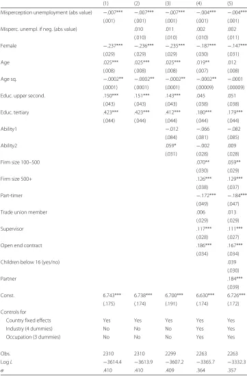
Tables 2 and 3 report the estimates of parametersβ andσ under different alternative model specifications. Robustness checks are presented in the Appendix, using the relative difference between the perceived and the actual unemployment rates or an alternative estimation method.
5 The impact of information misperceptions on wages
Table 2Interval regression, (log) wages on level of misperception of unemployment
(1) (2) (3) (4) (5)
Misperception unemployment (abs value) −.007*** −.007*** −.007*** −.004*** −.004***
(.001) (.001) (.001) (.001) (.001)
Misperc. unempl. if neg. (abs value) .010 .011 .002 .002
(.010) (.010) (.010) (.011)
Female −.237*** −.236*** −.235*** −.187*** −.147***
(.029) (.029) (.029) (.030) (.031)
Age .025*** .025*** .025*** .019** .012
(.008) (.008) (.008) (.007) (.008)
Age sq. −.0002** −.0002** −.0002** −.0002** −.0001
(.0001) (.0001) (.0001) (.00009) (.00009)
Educ. upper second. .150*** .151*** .143*** .045 .051
(.043) (.043) (.043) (.038) (.038)
Educ. tertiary .423*** .423*** .412*** .180*** .179***
(.044) (.044) (.044) (.044) (.044)
Ability1 −.012 −.066 −.082
(.084) (.081) (.085)
Ability2 .059* −.002 .009
(.031) (.028) (.028)
Firm size 100–500 .070** .059**
(.030) (.029)
Firm size 500+ .126*** .129***
(.038) (.037)
Part-timer −.172*** −.184***
(.049) (.047)
Trade union member .006 .013
(.029) (.029)
Supervisor .117*** .111***
(.028) (.027)
Open end contract .186*** .167***
(.034) (.034)
Children below 16 (yes/no) .039
(.030)
Partner .184***
(.039)
Const. 6.743*** 6.738*** 6.700*** 6.630*** 6.726***
(.175) (.174) (.191) (.174) (.172)
Controls for
Country fixed effects Yes Yes Yes Yes Yes
Industry (4 dummies) No No No Yes Yes
Occupation (3 dummies) No No No Yes Yes
Obs. 2310 2310 2299 2263 2263
LogL −3614.4 −3613.9 −3607.2 −3365.7 −3332.3
σ .410 .410 .409 .364 .357
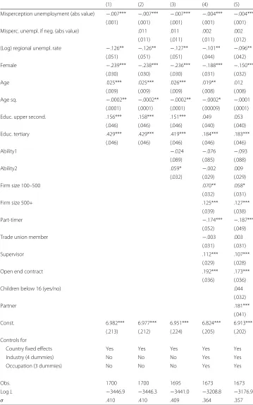
Table 3Interval regression, (log) wages on level of misperception of unemployment, including control for the regional unemployment rate
(1) (2) (3) (4) (5)
Misperception unemployment (abs value) −.007*** −.007*** −.007*** −.004*** −.004***
(.001) (.001) (.001) (.001) (.001)
Misperc. unempl. if neg. (abs value) .011 .011 .002 .002
(.011) (.011) (.011) (.012) (Log) regional unempl. rate −.126** −.126** −.127** −.101** −.096**
(.051) (.051) (.051) (.044) (.042)
Female −.239*** −.238*** −.236*** −.188*** −.150***
(.030) (.030) (.030) (.031) (.032)
Age .025*** .025*** .026*** .019** .012
(.009) (.009) (.009) (.008) (.008)
Age sq. −.0002** −.0002** −.0002** −.0002* −.0001
(.0001) (.0001) (.0001) (.00009) (.0001)
Educ. upper second. .156*** .158*** .151*** .049 .053
(.046) (.046) (.046) (.040) (.040)
Educ. tertiary .429*** .429*** .419*** .184*** .183***
(.046) (.046) (.046) (.046) (.046)
Ability1 −.024 −.076 −.093
(.089) (.085) (.088)
Ability2 .059* −.002 .009
(.032) (.029) (.029)
Firm size 100–500 .070** .058*
(.032) (.031)
Firm size 500+ .125*** .127***
(.039) (.038)
Part-timer −.174*** −.187***
(.052) (.049)
Trade union member −.003 .003
(.031) (.031)
Supervisor .112*** .107***
(.029) (.028)
Open end contract .192*** .173***
(.036) (.036)
Children below 16 (yes/no) .044
(.032)
Partner .181***
(.041)
Const. 6.982*** 6.977*** 6.951*** 6.824*** 6.913***
(.213) (.212) (.224) (.205) (.202)
Controls for
Country fixed effects Yes Yes Yes Yes Yes
Industry (4 dummies) No No No Yes Yes
Occupation (3 dummies) No No No Yes Yes
Obs. 1700 1700 1695 1673 1673
LogL −3446.9 −3446.3 −3441.0 −3208.8 −3176.9
σ .410 .410 .409 .364 .357
the worker’s broad occupation; whether the worker is a part-timer, performs a supervisor job, holds an open-ended contract, and is unionized). Finally, column 5 adds demographic controls (whether the worker lives with a partner and has any children). Whereas column 3 provides an indication on the impact of unemployment misperception on wages, col-umn 4 helps shed light on its mechanisms, as it controls for the attributes of the job the worker is matched to.
The impact of the regional unemployment rate on wages (Table 3) is remarkably in line with the wisdom established by the previous literature. Indeed, our results point to an elasticity of wages with respect to the regional unemployment rate ranging from−.127 to
−.096, whereas Blanchflower and Oswald (1994) derived the “law” of an elasticity of−.1. The interesting addition to the literature on misperceptions concerns our estimation of the impact of unemployment misperception on wages (line 1 in either Tables 2 or 3). We find that each percentage point misperception of the unemployment rate is associ-ated with a wage decline of 0.7 % (see the results in columns 1 to 3)—a misperception of the labor market situation by 10 p.p. would thus result in a wage penalty of 7 %, which is a noteworthy impact, in particular if one keeps in mind that the average mispercep-tion is 13 p.p. We further checked whether the impact could be different depending on whether the worker overshoots or undershoots when evaluating the country’s unemploy-ment rate. We would expect workers with a pessimistic view of the labor market to lower their reservation wages and thus earn lower wages; instead, workers with an optimistic view of the labor market could be overconfident and set too high reservation wages, though possibly having trouble finding a job. Consistent with that reasoning, we find that a pessimistic view of the labor market leads to lower wages. An optimistic view, instead, has no significant impact on wages (as indicated by a formal test on the sum of the esti-mated coefficients in lines 1 and 2 in each model specification), possibly due to the fact that very few of these workers underestimate the unemployment rate. Column 4 further introduces controls for job and employer attributes. Interestingly, the magnitude of the impact of labor market knowledge imperfections on wages is reduced—each percentage point misperception of the unemployment rate is now associated with a wage decline of 0.4 %—suggesting that part of the impact of misinformation on wages operates through worker matching to lower quality jobs.
In labor economics, information misperceptions fall under the category of “labor mar-ket frictions” that prevent or delay the matching of job vacancies and unemployed workers, according to search and matching models. However, both the theoretical and empirical modeling tend to bundle together frictions such as mobility costs, skill mis-matches, and lack of information on job requirements and wages offered or labor market tightness. Therefore, despite underlining the relevance of information flows, this line of literature has not so far analyzed the determinants of the role of inaccurate information per se.
and upper secondary education) (for an overview of the effect of educational levels on earnings, see Psacharopoulos 1994). Introducing controls for the worker ability as proxied by its capacity to understand the survey questions (column 3) does not change the sign or magnitude of the coefficients previously estimated, while pointing to a wage premium for more able workers (ability2); nevertheless, the impact of ability becomes non-significant once we account for the job characteristics, firm characteristics, and worker broad occu-pation. Larger firms pay higher wages. Part-time work is associated with lower wages, either because there is a penalty on hourly wages for part-time work or, by construction, when relying on earnings data instead of hourly wages. The impact of individual trade union membership, though positive, is not significant, as would be expected in European countries, where extension of collective bargaining contracts to non-unionized workers is widespread. Workers performing supervisory tasks earn a wage premium of
approxi-mately 12 %; those on open-ended contracts earn a wage premium of 21 %.11Married or
cohabiting workers earn higher wages, consistent with the literature on the marital-status wage premium (Blackburn and Korenman 1994). All of these estimates are very robust to the introduction of controls for the regional unemployment rate in Table 3. The fact that the estimates of the coefficients on the other variables included in the model fit remark-ably well the expectations drawn from the profusion of literature on wage regressions in general, and the regional wage curve in particular, points to the reliability of the procedure followed to infer earnings data from the ESS data.
5.1 Robustness checks
Robustness checks within the interval regression setting are presented in the Appendix Table 6. We depart from the regressions that included the control for the regional unemployment rate (Table 3) and consider the relative gap in the perception of the unem-ployment rate, computed according to Eq. 2, instead of the absolute gap. We consistently find that workers who have a pessimistic view of labor market opportunities earn lower wages, with an elasticity of wages with respect to the distance between perceived and actual unemployment rate of−.137 to−.093. Moreover, we still find that an optimistic view of labor market opportunities has no significant impact on wages (formal tests on the sum of the coefficients in the two first lines of each model). The regional unemploy-ment elasticity of pay changes little, just like the estimated coefficients on all other control variables.
5.2 A potential mechanism? Misperceptions of the labor market situation and worker’s career decisions
A gap between the country’s unemployment rate perceived by a worker and the actual unemployment rate provides a measure of misunderstanding of the degree of labor mar-ket tightness by the worker. This misperception is bound to affect individual behavior in the labor market—to the extent that a pessimistic view is associated with concern over becoming unemployed, it is expected to influence decisions such as that on the reservation wage. Whereas there is no data available that would enable a full test of this hypothesis, we can nevertheless explore whether the misperception of the unemployment rate is associated with an individual’s expectation of becoming unemployed. Such evi-dence would provide a possible channel for the misperceptions on the situation of the labor market to impact wages.
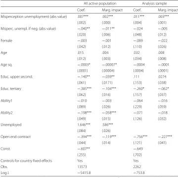
Participants in the survey were asked, “how likely it is that during the next 12 months you will be unemployed and looking for work for at least four consecutive weeks?” (ESS 2008c, p. 35). The possible answers were the following: very likely, likely, not likely, and not at all likely. We generate a dummy variable that takes value one if the answer was “very likely” or “likely” and zero otherwise. We estimate the probability of a positive answer as a function of the unemployment misperception and a set of covariates, con-trolling for country fixed effects. The covariates include the actual unemployment rate in the country (which varies depending on the survey month) and the worker’s age, gender, education, and ability, as well as her current labor market status (dummy for unemployed, with employed as the omitted category, and a dummy with value one if the individual is employed on a permanent contract and zero otherwise). This set of regressors replicates those in our major specification of the wage model, in column 3 of Table 2, augmented to include the job attribute that is expected to have a direct impact on perceptions of future unemployment, namely the duration of the current employment contract (open-ended, as opposed to short duration). The regressions were run both on the sample of active popu-lation (in which case, we further control for the current unemployment status) and on the analysis sample, which includes only employed workers. Results are reported in Table 4.
For the active population, the covariates that describe the working status have signs aligned with expectations. Being unemployed increases the most the perceived likelihood of future unemployment. Having a permanent contract points in the opposite direction, even though the absolute magnitude of the effect is smaller. More educated individu-als show less concern over the possibility of being unemployed. No significant gender differences are detected.
The coefficient of the unemployment misperception is significant and positive—the overestimation of the unemployment rate is associated with a higher perceived probability of being unemployed in the near future. Conversely, the underestimation of the country’s unemployment rate is associated with a lower perceived probability of being unemployed in the near future (though significant only at the 10 % level).
Table 4Perceived probability of being unemployed within the next 12 months, probit model
All active population Analysis sample
Coef. Marg. impact Coef. Marg. impact
Misperception unemployment (abs value) .007*** .002*** .011*** .003***
(.002) (.000) (.004) (.001)
Misperc. unempl. if neg. (abs value) −.040** −.011** −.024 −.005
(.020) (.006) (.048) (.012)
Female −.003 −.001 −.089 −.022
(.042) (.012) (.110) (.026)
Age .015 .004 .032 .008
(.012) (.003) (.034) (.008)
Age sq. −.0003* −.00007* −.0004 −.0001
(.0001) (.00004) (.0004) (.0001)
Educ. upper second. −.140** −.039** .111 .0274
(.061) (.0171) (.153) (.038)
Educ. tertiary −.385*** −.104*** −.260* −.062*
(.062) (.016) (.157) (.037)
Ability1 −.010 −.003 −.064 −.016
(.089) (.026) (.229) (.059)
Ability2 −.198*** −.058*** −.071 −.018
(.049) (.015) (.126) (.032)
Unemployed 1.646*** .586***
(.084) (.026)
Open end contract −.394*** −.119*** −.756*** −.227***
(.044) (.014) (.121) (.041)
Const. −.607** −.649
(.255) (.702)
Controls for country fixed effects Yes Yes
Obs. 13573 2262
LogL −5415.8 −753.8
Source: Computations are based on ESS (2008). Notes: The model uses ESS post-stratification weights combined with population size weights. Robust standard errors are in parenthesis. Columns 1 and 2 are computed on the active population sample (employed and unemployed respondents) in the 16 countries under analysis; columns 3 and 4 are computed on the analysis sample of employed workers. Marginal impacts are computed at the mean values and considering the change in each dummy variable from zero to one. Asterisks indicate statistically significant parameters at *10 %, **5 %, and ***1 % levels
These results suggest that the misperception of a national phenomenon—the coun-try unemployment rate—is associated with expectations about one’s own labor market prospects. Therefore, the information gap is likely to affect labor market choices, in particular the definition of the wage threshold for a job offer to be deemed acceptable.
exploit this information friction, having more bargaining power that would allow them to offer lower wages.
6 Conclusions
We contribute to the empirical literature on the impact of misperceptions, by showing that they affect an individual’s actual labor market outcomes. We estimate wage regres-sions including worker attributes, as well as firm and job attributes, augmented to include our key variable of interest, the degree of misperception by the worker of the labor mar-ket tightness. We adopt a threefold strategy to tackle potential endogeneity problems: controlling for worker ability, including country fixed effects, and controlling for the unemployment rate in the region of residence.
Our results lend support to the claim that a worker’s knowledge of labor market con-ditions is crucial: “The information a man possesses on the labor market is capital: it was produced at the cost of search, and it yields a higher wage rate than on average would be received in its absence” (Stigler 1962, p. 103). We find that workers’ pessimistic view of the labor market situation lowers their wages—-each 1 percentage point deviation of the perceived unemployment rate from the actual one translates into a reduction in wages of 0.7 % (0.4 % once we control for job and employer attributes). This result is very robust to alternative specifications of the model. In turn, an optimistic view of the labor market has no significant impact on wages. We discuss possible mechanisms driving these results. An overestimation of the unemployment rate leads to concern over one’s own future employ-ment prospects and is therefore likely to reduce perceived bargaining power, lowering reservation wages; its underestimation, on the contrary, could raise reservation wages, but it would render job finding more difficult.
Endnotes
1In the terminology of the data producer, we have used the Integrated File that merges
all countries with comparable data, edition 4.3.
2We used weighted data when computing these percentages of non-response items.
3Results on the probit model estimated are available from the authors upon request.
4Belgium, Denmark, Estonia, Finland, France, Germany, Hungary, Ireland, Latvia, The
Netherlands, Norway, Poland, Romania, Slovenia, Sweden, and the UK.
5Working age: the age from which people are legally entitled to work up to retirement
age. Unemployed: people who cannot find paid work (ESS 2008c, p. 25). We disregard the subtlety that the total population is the denominator respondents were asked to con-sider, instead of the active population, as we believe the question was phrased in the simplest and least technical way possible to capture the respondent’s perception of the unemployment rate.
6Defined as the start of the interview (which coincides with the end moment in
virtually all cases).
7We implemented yet another robustness check. According to our core index of
on wages using this alternative index. Results do not change (no coefficient changes its significance level, and the few coefficients that change magnitude do so at the third decimal place). These results are available from the authors upon request.
8 NUTS—Nomenclature of Territorial Units for Statistics.
9 The estimation sample includes both the employed and unemployed population, as it
seems a more sensible sample on which to evaluate the determinants of unemployment misperceptions. Estimation on the analysis sample of employed workers yields coeffi-cients with the same sign, similar magnitudes, but non-significant results on ability and the regional unemployment rate.
10We have also computed the gap between the perceived unemployment rate and the
regional unemployment rate (instead of the national). We find that both gaps are highly correlated (coefficient above .98) and a formal test cannot reject the equality of their means.
11Either one computed as exp(β)−1.
12The coefficient on the negative misperception (line 2) is very imprecisely estimated.
Therefore, we cannot reject the hypothesis that the impact of the underestimation of the unemployment rate is zero (sum of the coefficients in lines 1 and 2), just like we cannot reject that it is equal to the impact of overestimation of the unemployment rate.
Appendix
Table 5Misperceptions of unemployment, interval regression
(1) (2)
Educ. upper second. −4.179*** −4.063***
(.542) (.541)
Educ. tertiary −7.763*** −7.810***
(.548) (.549)
Ability1 −3.030*** −3.012***
(.886) (.890)
Ability2 −1.662*** −1.678***
(.452) (.453)
Unemployed 5.604*** 5.799***
(.758) (.755)
Female 4.762*** 4.786***
(.357) (.357)
Age −.514*** −.510***
(.096) (.096)
Age sq. .005*** .005***
(.001) (.001)
Region. unempl. rate .321***
(.058)
Diff. reg. and national unempl. rate (abs. value) .237**
(.098)
Const. 30.192*** 31.857***
(2.119) (2.108)
Obs. 10506 10506
LogL −31981.8 −32000.9
σ 12.9 12.9
Table 6Interval regression, (log) wages on (log) misperception of unemployment, including control for the regional unemployment rate
(1) (2) (3) (4) (5)
(Log) ratio misperc. unempl. (abs value) −.132*** −.137*** −.136*** −.093*** −.098***
(.023) (.023) (.024) (.022) (.022)
(Log) ratio misp. unemp. if neg. (abs value) .110** .110** .054 .056 (.046) (.046) (.045) (.048) (Log) regional unempl. rate −.128** −.127** −.128** −.102** −.096**
(.051) (.051) (.050) (.044) (.043)
Female −.239*** −.235*** −.233*** −.185*** −.146***
(.030) (.030) (.030) (.031) (.032)
Age .025*** .025*** .026*** .019** .012
(.009) (.009) (.009) (.008) (.008)
Age sq. −.0002** −.0002** −.0002** −.0002* −.0001
(.0001) (.0001) (.0001) (.00009) (.0001)
Educ. upper second. .158*** .158*** .150*** .047 .051
(.046) (.046) (.046) (.040) (.040)
Educ. tertiary .433*** .428*** .416*** .181*** .179***
(.047) (.046) (.046) (.046) (.046)
Ability1 −.012 −.069 −.085
(.087) (.084) (.087)
Ability2 .062* −.0008 .011
(.032) (.029) (.029)
Firm size 100–500 .069** .057*
(.032) (.031)
Firm size 500+ .126*** .129***
(.039) (.038)
Part-timer −.175*** −.188***
(.052) (.049)
Trade union member −.003 .004
(.031) (.031)
Supervisor .114*** .109***
(.029) (.028)
Open end contract .193*** .174***
(.036) (.036)
Children below 16 (yes/no) .043
(.032)
Partner .182***
(.041)
Const. 7.007*** 7.009*** 6.971*** 6.842*** 6.932***
(.214) (.213) (.225) (.206) (.203)
Controls for
Country fixed effects Yes Yes Yes Yes Yes
Industry (4 dummies) No No No Yes Yes
Occupation (3 dummies) No No No Yes Yes
Obs. 1700 1700 1695 1673 1673
LogL −3450.9 −3447.1 −3441.5 −3207.1 −3174.8
σ .411 .410 .409 .364 .356
Table 7Ordered probit, (log) wages on level of misperception of unemployment, including control for the regional unemployment rate
(1) (2) (3) (4) (5)
Misperception unemployment (abs value) −.017*** −.016*** −.016*** −.012*** −.013***
(.003) (.003) (.003) (.003) (.003)
Misperc. unempl. if neg. (abs value) .034 .034 .010 .010
(.027) (.027) (.030) (.033) (Log) regional unempl. rate −.304** −.305** −.307** −.274** −.263**
(.126) (.126) (.125) (.123) (.120)
Female −.573*** −.570*** −.566*** −.502*** −.409***
(.071) (.071) (.071) (.082) (.087)
Age .058*** .058*** .060*** .049** .030
(.022) (.022) (.022) (.022) (.023)
Age sq. −.0005** −.0005** −.0006** −.0005* −.0002
(.0003) (.0003) (.0003) (.0003) (.0003)
Educ. upper second. .367*** .372*** .354*** .115 .131
(.114) (.114) (.113) (.112) (.114)
Educ. tertiary 1.033*** 1.035*** 1.010*** .500*** .510***
(.118) (.118) (.118) (.126) (.130)
Ability1 −.019 −.163 −.211
(.211) (.228) (.241)
Ability2 .129* −.025 .005
(.078) (.080) (.082)
Firm size 100–500 .207** .177**
(.086) (.085)
Firm size 500+ .342*** .357***
(.104) (.103)
Part-timer −.490*** −.541***
(.142) (.137)
Trade union member .032 .051
(.083) (.084)
Supervisor .306*** .298***
(.079) (.078)
Open end contract .556*** .515***
(.101) (.102)
Children below 16 (yes/no) .144
(.090)
Partner .488***
(.114) Controls for
Country fixed effects Yes Yes Yes Yes Yes
Industry (4 dummies) No No No Yes Yes
Occupation (3 dummies) No No No Yes Yes
Obs. 1700 1700 1695 1673 1673
LogL −3420.7 −3419.8 −3414.9 −3177.1 −3145.1
IZA
Journal
o
fL
abor
Policy
(2016) 5:13
Page
21
of
22
Table 8Marginal effects ordered probit, (log) wages on level of misperception of unemployment, including control for the regional unemployment rate
Interval1 Interval2 Interval3 Interval4 Interval5 Interval6 Interval7 Interval8 Interval9 Interval10
(1) 0.00076 0.00206 0.00245 0.00131 −0.00017 −0.00095 −0.00152 −0.00150 −0.00128 −0.00116
0.00017 0.00038 0.00048 0.00028 0.00010 0.00021 0.00031 0.00031 0.00025 0.00025
(2) 0.00073 0.00199 0.00238 0.00127 −0.00016 −0.00092 −0.00147 −0.00145 −0.00124 −0.00113
0.00017 0.00038 0.00048 0.00028 0.00010 0.00021 0.00031 0.00031 0.00025 0.00025
(3) 0.00072 0.00198 0.00237 0.00127 −0.00016 −0.00092 −0.00147 −0.00145 −0.00123 −0.00111
0.00017 0.00038 0.00048 0.00028 0.00010 0.00020 0.00031 0.00031 0.00025 0.00025
(4) 0.00030 0.00129 0.00198 0.00111 −0.00019 −0.00085 −0.00125 −0.00109 −0.00078 −0.00052
0.00010 0.00035 0.00055 0.00032 0.00010 0.00025 0.00035 0.00032 0.00021 0.00016
(5) 0.00030 0.00136 0.00216 0.00119 −0.00026 −0.00096 −0.00137 −0.00115 −0.00079 −0.00049
0.00009 0.00035 0.00057 0.00033 0.00012 0.00027 0.00037 0.00032 0.00020 0.00014
Competing interests
The IZA Journal of Labor Policy is committed to the IZA Guiding Principles of Research Integrity. The authors declare that they have observed these principles.
Acknowledgements
We are grateful to David Card, Paulo Guimaraes, Louis-Philippe Morin, and an anonymous referee for comments at different stages of this project. Cardoso acknowledges the support of the Spanish Ministry of the Economy and Competitiveness (grant ECO2012-38460 and the Severo Ochoa Programme for Centres of Excellence in R&D SEV-2011-0075) and theGeneralitat de Catalunya, grant 2014-SGR-1414. Loviglio acknowledges the support of La Caixa Foundation. The authors declare that they have no conflict of interest.
Responsible editor: Juan Jimeno
Author details
1IAE-CSIC, Campus UAB, 08193 Bellaterra, Spain.2Universitat Autònoma de Barcelona, Campus UAB, 08193 Bellaterra,
Spain.
Received: 23 February 2016 Accepted: 31 March 2016
References
Blackburn MK, Korenman S (1994) The declining marital-status earnings differential. J Popul Econ 7(3):247–270 Blanchflower DG, Oswald AJ (1994) The wage curve. MIT Press, Cambridge, MA
Blanchflower DG, Kelly R (2008) Macroeconomic literacy, numeracy and the implications for monetary policy. Mimeo, Speech at the Bank of England, April 29
Cameron CA, Trivedi PK (2005) Microeconometrics: methods and applications. 2nd edition. Cambridge University Press, Cambridge
Conover PJ, Feldman S, Knight K (1986) Judging inflation and unemployment: the origins of retrospective evaluations. J Polit 48(3):565–588
Curtin R (2008) What U.S. consumers know about economic conditions. In: Statistics, Knowledge and Policy 2007: Measuring and Fostering the Progress of Societies. OECD, Paris. pp 153–176
Diamond PA (1982) Wage determination and efficiency in search equilibrium. Rev Econ Stud 49(2):217–27 Duffy D, Lunn PD (2009) The misperception of inflation by Irish consumers. Econ Soc Rev 40(2):139–163
European Social Survey [ESS] Round 4 Data (2008) Data file edition 4.3. Norwegian Social Science Data Services, Norway, Data Archive and Distributor of ESS data
European Social Survey [ESS] (2008a) European Social Survey (2008) Data Protocol, Edition 1.2. Bergen European Social Survey Data Archive, Norwegian Social Science Data Services
European Social Survey [ESS] (2008b) European Social Survey (2008) Project Instructions. Bergen European Social Survey Data Archive, Norwegian Social Science Data Services
European Social Survey [ESS] (2008c) European Social Survey (2008) Source Questionnaire Amendment 03 (Round 4, 2008/9). Bergen European Social Survey Data Archive, Norwegian Social Science Data Services
European Social Survey [ESS] (2010) ESS-4 2008 Documentation report. Edition 5.1. Bergen European Social Survey Data Archive, Norwegian Social Science Data Services
Eurostat (2013) Harmonised unemployment rates (%)—monthly data. http://ec.europa.eu/eurostat/web/products-datasets/-/ei_lmhr_m. Accessed August 2013
Eurostat (2014) Unemployment rate by NUTS 2 regions. http://ec.europa.eu/eurostat/web/products-datasets/-/ tgs00010. Database queries on unemployment rate by NUTS1 and NUTS2. Accessed June 2014
Fullone F, Gamba M, Giovannini E, Malgarini M (2008) What do citizens know about statistics? The results of an OECD/ ISAE survey on Italian consumers. In: Statistics, Knowledge and Policy 2007: Measuring and Fostering the Progress of Societies. OECD, Paris. pp 197–212
Hoffmeyer-Zlotnik JHP, Warner U (2006) Methodological discussion of the income measure in the European social survey round 1. Metodoloski Zvezki Adv Methodol Stat 3(2):289–334
Ipsos MORI (2014) Perceptions are not reality: things the world gets wrong. Website https://www.ipsos-mori.com/ researchpublications/researcharchive/3466/Perceptions-are-not-reality-10-things-the-world-gets-wrong.aspx. Accessed May 13, 2015
Kunovich RM (2013) Perceived unemployment: the sources and consequences of misperception. Int J Sociol 42(4):100–123
Micklewright J, Schnepf SV (2010) How reliable are income data collected with a single question. J R Stat Soc Series A 173(2):409–429
Moore RE, Baker Kearfott R, Cloud MJ (2009) Introduction to interval analysis. Society for Industrial and Applied Mathematics, Philadelphia
Orland A (2013) Personality traits and the perception of macroeconomic indicators—survey evidence. Working Paper Ruhr Economic Papers, 0424. Bochum: Rheinisch-Westfaelisches Institut fuer Wirtschaftsforschung
Papacostas A (2008) Special Eurobarometer Europeans knowledge on economical indicators. In: Statistics, Knowledge and Policy 2007: Measuring and Fostering the Progress of Societies. OECD, Paris. pp 177–196