C A S E S T U D Y
Open Access
Airline new customer tier level forecasting for
real-time resource allocation of a miles program
Jose Berengueres
1*and Dmitry Efimov
2* Correspondence:[email protected] 1
UAE University, 17551 Al Ain, Abu Dhabi, UAE
Full list of author information is available at the end of the article
Abstract
This is a case study on an airline’s miles program resource optimization. The airline had a large miles loyalty program but was not taking advantage of recent data mining techniques. As an example, to predict whether in the coming month(s), a new passenger would become a privileged frequent flyer or not, a linear extrapolation of the miles earned during the past months was used. This information was then used in CRM interactions between the airline and the passenger. The correlation of extrapolation with whether a new user would attain a privileged miles status was 39% when one month of data was used to make a prediction. In contrast, when GBM and other blending techniques were used, a correlation of 70% was achieved. This corresponded to a prediction accuracy of 87% with less than 3% false positives. The accuracy reached 97% if three months of data instead of one were used. An application that ranks users according to their probability to become part of privileged miles-tier was proposed. The application performs real time allocation of limited resources such as available upgrades on a given flight. Moreover, the airline can assign now those resources to the passengers with the highest revenue potential thus increasing the perceived value of the program at no extra cost.
Keywords:Airline; Customer equity; Customer profitability; Life time value; Loyalty program; Frequent flyer; FFP; Miles program; Churn; Data mining
Background
Previously, several works have addressed the issue of optimizing operations of the air-line industry. In 2003, a model that predicts no-show ratio with the purpose of opti-mizing overbooking practice claimed to increase revenues by 0.4% to 3.2% [1]. More recently, in 2013, Alaska Airlines in cooperation with G.E and Kaggle Inc., launched a $250,000 prize competition with the aim of optimizing costs by modifying flight plans [2]. However, there are very little works on miles programs or frequent flier programs that focus on enhancing their value. One example is [3] from Taiwan, but they focused on segmenting customers by extracting decision-rules from questionnaires. Using a
Rough Set Approach they report classification accuracies of 95%. [4] focused on
seg-menting users according to return flight and length of stays using a k-means algorithm. A few other works such as [5], focused on predicting the future value of passengers (Customer Equity). They attempt to predict the top 20% most valuable customers. Using SAS software they report false positive and false negative rate of 13% and 55% respectively. None of them have applied this knowledge to increase the
proposition of miles programs. All this in spite the fact that some of these programs have become more valuable than the airline that started them. Such is the case of Aeroplan, a spin off of the miles programs started by Toronto based Air Canada. Air Canada is as of today valued at $500 M whereas Aeroplan is valued at $2bn, four times more [6]. Given this it is surprising that so many works focus in ticket or “revenue management” [7] but few focus on their miles programs. In this case study we report the experience gained when we analyzed the data of an airline’s miles program. We show how by applying modern data mining techniques it is pos-sible to create value for both: (1) the owner of the program and (2) future high-value passengers.
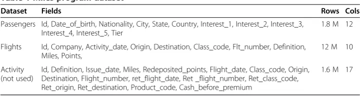
The data of the miles program was provided by Etihad Airlines and was 1.2GBytes in size when zip compressed. It contained three tables of anonymized data from year 2008 to 2012, corresponding to about 1.8 million unique passengers. The tables contain the typical air miles program data such as:
1. Age and demographics. 2. Loyalty program purchases etc. 3. Flight activity, miles earned etc.
Case Description
Objective
After co-examining the opportunities that the data offered with the airline we decided to focus on high-value passengers with the objective to: predict and discriminate which of the new passengers who enroll the miles program will be high-value customers before it is obvious to a human expert.
Rationale
Business justification:
1. So that potential high-value customers are identified in order to gain their loyalty sooner. 2. So that limited resources such as upgrades are optimally allocated to passengers
with potential to become high-value. 3. To enhance customer profiling.
Current method: linear extrapolation
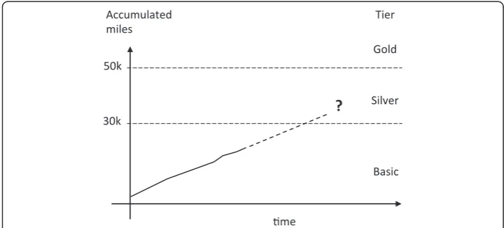
The miles program was using three main tiers to classify customer by value. Ordered form less to more value these are: basic, silver, gold. The airline was using the following method to predict future tier status: a passenger flight activity is observed on a monthly basis then, a linear extrapolation on how much they will fly in the coming month(s) is performed (Figure 1). This information was then used in interactions with customers.
Definition of the target variable
whether they will attain Silver or greater tier status within S additional days after day D. We will later refer to this binary variable as silver_attain, and to this model as D/S model. Then past behavior of customers is feed into the model. The model is described further in the text.
Identifying future high value customers
When a new customer joins the program, (and D days have passed since then) the model can be used to make a prediction about the likelihood that they will become Silver in the near or far future. Figure 2 and Table 1 show examples. For business
Figure 1How the airline uses extrapolation to predict when/or if a customer will become high-value customer.Y-axis, accumulated miles earned by a given customer. X-axis, time. Dashed-line prediction.
D
S
Silver
before now
purposes we equate Silver tier status with high-value customer. However, this hy-pothesis was not validated in the scope of the project.
Previous to model construction we performed two actions:
1) Cleaning of the data. 2) Feature extraction.
Cleaning
Initially, we had three tables: Passengers, Flights and Activity. Activity, which contains data related to miles transactions, was not used because it did not help improve re-sults. The Airline suggested that this might be due to incompleteness of data. For example, by Airline policy all monetary transactions were unavailable to us and had been removed from datasets. Table 1 shows the list of fields for each table. First we removed two outlier cases for passengers whose future tier prediction is straight-forward or has little merit:
1) Passengers who fly less than one return trip in six years.
2) Passengers with very high activity (number of flights greater than 500).
Additionally, before the data was handed over to us, the airline anonymized the id field. The id had been replaced by an alphanumeric hash code of length 32 charac-ters long. We changed these cumbersome hash ids into integer numerical values to increase the performance. Big datasets made it very difficult for R Language to ope-rate with hash ids during feature engineering.
Feature extraction
The system works in the following way: For each passenger a vector is constructed considering data pertaining to the D period only. For example, if D= 15 days, then the flights and data we would consider to build the aforementioned vector are any flights between start_date and start_date +D, where start_date is the first flight date of a new passenger. Note that start_date varies for every passenger. Now for each passenger we construct a vector that depends on three variables:
1) The passenger data in the Tables. 2) start_date.
3) Length ofD.
Table 1 Miles program dataset
Dataset Fields Rows Cols
Passengers Id, Date_of_birth, Nationality, City, State, Country, Interest_1, Interest_2, Interest_3, Interest_4, Interest_5, Tier
1.8 M 12
Flights Id, Company, Activity_date, Origin, Destination, Class_code, Flt_number, Definition, Miles, Points,
12 M 10
Activity (not used)
Id, Definition, Issue_date, Miles, Redeposited_points, Flight_date, Class_code, Origin, Destination, Flight_number, ret_flight_date, Ret _flight_number, Ret_class_code, Ret_origin, Ret_destination, Product_code, Cash_before_premium
Each component of the vector is called a “feature”. The length of the vector is 634 features. The vector is equivalent to a digital fingerprint for each passenger considered in a given period. Some features are straightforward to calculate and others require complex calculations. Following we explain how each feature was calculated. We have divided the features in three groups: metric, categorical and cluster features.
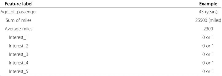
Group 1 - Metric features
A metric feature is data that is already in numerical format. For example, age of a customer.
Group 2 - Categorical features
A categorical feature is a text variable, the content of which can only belong to a finite group of choices. The column “City” is such an example. The main problem with ca-tegorical variables is that they must be converted to numbers somehow. Since a com-puter does not understand “city names”per se, there are different ways to operate with such variables. One way is to encode code each name (aka level or category) of each categorical variable into a binary feature. Therefore, we opted for an interpretation of categorical variables using the dummy variable method as follows:
Let N be the total number of values for a given categorical variable, then we create N new“dummy”features. If a given record has value = ithlevel, then the ithdummy feature equals 1, otherwise 0.
Unfortunately, this transformation restricts range of algorithms that are effective: algorithms based on metrical approach such as SVM [8] yield poor results in such cases.
One of such features is: “city” (Cities to where the passenger has flown during D, from the table flights). Following, we explain an example on how the categorical city
variable was processed. Each city to where the airline flies is represented as a feature in the vector. If the given passenger did not fly even once to the given city during D, then the feature is set to 0, if it flew one or more times it is set to 1. The same process is performed for Class tickets letters. The categorical variables that are exploded to binary format using the dummy method are:
1) Passenger Nationality. 2) City of Passenger’s address. 3) State of Passenger’s address. 4) Country of Passenger’s address. 5) Passenger’s Company (Employer). 6) Flight Origin (Airport).
7) Flight Destination (Airport).
8) Ticket Class Code (Economy E, F, K…).
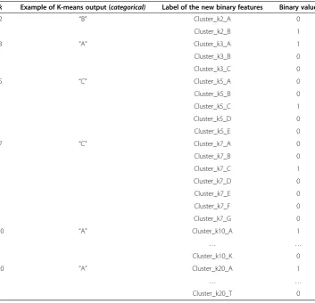
Group 3. Cluster features
Once all categorical features are converted to binary ones, even if their quantity has in-creased, it is possible to apply clustering algorithms to identify groups of passengers with similar associated“vectors”. In this case, we applied the tried and proven k-means algorithms with different number of clusters (2, 3, 5, 7, 10, 15, and 20) to classify all passengers in clusters. The kdenotes the number of clusters. So for example is k = 3 it means there are 3 clusters (A, B, C). Every passenger vector will be assigned to the
“closest” cluster center as defined by Euclidean distance in n-dimensions, where n is the number of features of the vectors. At this point a cluster label (“A”, “B” or“C”) is assigned to each passenger vector. Then as before we use the dummy variable method to explode cluster labels into binary features. This was done in the following way: For each passenger all previous features (of Tables 3 and 2) are put in vector form. Then, if we are considering 100 passengers, and data of say 354 flights that satisfy the condition of belonging in the D period, then we produce 100 vectors. This is input into a k-means algorithm for k = 3. k denotes de number of clusters into which the vectors will be classified. The algorithm will attempt to classify each of the 100 vectors into k = 3 clusters, A or B or C. Using the dummy variable method we generate three new variables: Cluster_k3_A, Cluster_k3_B, Cluster_k3_C. These 3 variables will become new additional features instead of a categorical feature that says (“A”,“B”or“C”). Then if a vector (passenger) belongs to “A”, its Cluster_k3_A feature is set to 1 and 0 other-wise, conversely, if the vector belongs to“B”then only Cluster_k3_B is set to 1, and so on. This process is repeated for k = 2, 5, 7, 10, 15, 20. Table 4, shows the features and
Table 2 Example of conversion from categorical to binary for a given passenger
Feature label Example value
City_1 (Amsterdam) 0
City_2 (Barcelona) 1
… …
City_323 (Zagreb) 1
Class_code_1 (“A”) 0
Class_code_2 (“B”) 1
Class_code_3 1
Class_code_45 (“Z”) 0
Table 3 Metric features
Feature label Example
Age_of_passenger 43 (years)
Sum of miles 25500 (miles)
Average miles 2300
Interest_1 0 or 1
Interest_2 0 or 1
Interest_3 0 or 1
Interest_4 0 or 1
Interest_5 0 or 1
an example where a passenger vector has been classified into cluster “B” for k = 2, cluster“A”for k = 3 etc…
After all this process, for each passenger vector, we add these binary cluster fea-tures to the corresponding passenger vector. Table 5 shows an example. At this point it should be clear the label assigned to each feature is irrelevant. The order of the features is also irrelevant, only maintaining a consistent ordering of features in the vectors is important. Naturally, the more training vectors available, the more ac-curate the predictions can be. We used 50,000 vector examples to train the model. A benefit of feeding clustered features to a model is that it could help to find high order relationships between similar data points. We use a GBM model that accounts for up to 5-degree relations.
Target variable
Once the vectors for each passenger are generated we need to define the target variable. This is the variable that we want to predict. In our case, the variable is 1 if the user became Silver tier during the S period as shown in Figure 2 and 0 otherwise. To generate training
Table 4 Example of creation of 60 cluster features by the dummy method
k Example of K-means output (categorical) Label of the new binary features Binary value
2 “B” Cluster_k2_A 0
Cluster_k2_B 1
3 “A” Cluster_k3_A 1
Cluster_k3_B 0
Cluster_k3_C 0
5 “C” Cluster_k5_A 0
Cluster_k5_B 0
Cluster_k5_C 1
Cluster_k5_D 0
Cluster_k5_E 0
7 “C” Cluster_k7_A 0
Cluster_k7_B 0
Cluster_k7_C 1
Cluster_k7_D 0
Cluster_k7_E 0
Cluster_k7_F 0
Cluster_k7_G 0
10 “A” Cluster_k10_A 1
… …
Cluster_k10_K 0
20 “A” Cluster_k20_A 1
… …
Cluster_k20_T 0
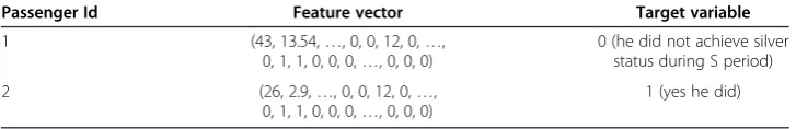
Table 5 Example of feature vectors generated per each passenger
Passenger Id Example vector
examples we use samples from past years and check what happened to them. This set of vectors and associated target variables constitutes a training set. Table 6 shows an example of passenger vectors from Table 5 with the corresponding target variable.
Now, we can consider all this vectors as a matrix, where rows are passengers, col-umns are features, and the last column is the target variable. We will use such a matrix to train a mathematical model with the purpose of predicting the target variable in new passengers. Once the model is trained, to predict if a passenger will attain silver status in a given time frame S (in the future) we only need to generate its feature vector by observing the passenger for a period of time D since their first flight. Once the vector is generated (naturally, without target variable) we can input it into the model and the model will output a number. There are no restrictions on when to ask a model for a prediction as long as the data for the given S period is available.
Model
The high nonlinearity of the features (meaning low correlation between target variable and features) restricts the number of algorithms we can use to predict with high accur-acy. We chose to blend two algorithms, which were in our opinion the most appropri-ate for this dataset: the GBM (Generalized Boosting Machine package) and GLM (Generalized Linear Model, glm in R). Both models are trained with the same target variable:silver_attain,and try minimize the binomial deviance (Log Loss) of prediction error. While, we chose GLM and GBM because they produce different models, GLM can be considered as non-parametric version of GBM.
GBM
The aforementioned training matrix was used to train a GBM model in R Language. This is convenient because an implementation of GBM is available as an open source library in R, so we don't need to code it from scratch. GBM has various parameters that can affect the performance of the model. For example, the number of trees (size) is one of them and usually the most important. Manual grid search was performed to determine the optimal parameter values. 75% of the data was used to train a model and 25% was used to test the prediction. The optimal GBM parameters were:
1) distribution =“bernoulli”, 2) n.trees = 2000,
3) shrinkage = 0.01, 4) interaction.depth = 0.5, 5) bag.fraction = 0.5, 6) train.fraction = 0.1, 7) n.minobsinnode = 10.
Table 6 Example of feature vectors and target variables
Passenger Id Feature vector Target variable
1 (43, 13.54,…, 0, 0, 12, 0,…, 0, 1, 1, 0, 0, 0,…, 0, 0, 0)
0 (he did not achieve silver status during S period) 2 (26, 2.9,…, 0, 0, 12, 0,…,
0, 1, 1, 0, 0, 0,…, 0, 0, 0)
A good description of the GBM implementation we used can be found in [9]. It works as follows: the training matrix is used to train the model with the aforemen-tioned parameters. After, some minutes we have a trained model. Now to make a new prediction on a passenger vector or a number of passenger vectors, we input it in the model and the model will return a number from 0 to 1 for each passenger vec-tor. 0 means that the model predicts 0% chance for that passenger to attain silver tier status within the S period of time. A 1 means that the model is the most confident the silver tier will be attained. Training the model takes about 1 hour, but asking the model to predict what will happen to 10,000 passengers takes just seconds.
GLM
The other algorithm used is GLM. GLM stands for General Linear Model. As before we used the implementation in R Language provided by [10]. GLM is just a simple logistic regression where we optimize binomial deviance, whereError = silver_attain– pre-diction.Default parameters where used except for family which was set to“binomial”.
Blending with grid search
Combining predictions is known to improve accuracy if certain conditions are met [11]. In general, the less correlation between the individual predictors, the higher the gain in accuracy. A way that usually lowers cross-correlation is to combine models of different“nature”. We chose to combine a decision tree based algorithm (GBM) and regression based one (GLM). For a 3/3 model the relative gain in accuracy due to blending was 3%. The final prediction was constructed as a linear combination of the output of the two. Grid search was used to find which linear combination was opti-mal on the training set. The optiopti-mal combination was 90% of the GBM prediction plus 10% of the GLM prediction.
Loss function
A natural way to estimate the error in problems where the target variable is binary is the use of Precision and Recall so we can account for the number of false positives and false negatives. However, one of the exceptional properties of the target variable (silver_attain) was the huge number of 0’s and small number of 1’s. This is hardly surprising: after all, by design, only a small percentage of the total passengers are supposed to attain a privileged tier. Another interesting fact is that the airline desired to determine future silver and gold passengers with highest possible accuracy; this is, a low false positive rate (mistakes). However, since the penalty cost for false negatives is not high, the acceptable precision level can be lower. These two observations enabled us to modify the usual definition of Precision and Accuracy in the following way:
P¼ N0 N0þN1
A¼ N0
N0þN2 ð
1Þ
silver and who indeed became silver. In the next section we will show the calculated error for the normal Precision and Recall and the calculated error according to chosen loss functions (Eq.1).
Discussion and evaluation
It takes about 18 hours on a laptop to clean the data and construct the features. To build a D/S model takes about 1 hour per each D/S combination. Once a model is pre-calculated, making a prediction for one single passenger takes less than 350 ms (similar to a Google search).
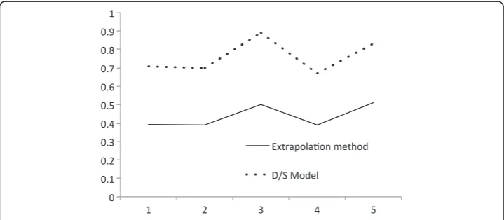
Compared performance
Figure 3, Tables 7 and 8 compare key performance indicators of predictive power be-tween the previous model used by the airline (monthly extrapolation) and the D/S model. The columns P and A of Table 7 were calculated according to Eq. 1. Table 8 shows actual numbers on one particular example for D/S = 3/3 months respectively. Table 8 also shows why the calculation of Precision and Accuracy in the usual way is not suitable to assess model performance on the given dataset because of huge number of 0's. A trade-off between Accuracy, Precision, D and S clearly exists. These parame-ters can be adjusted to suit various forecasting needs. Additionally, Table 7 data shows that accuracy is, roughly speaking, inversely proportional to the length of S. This is, the longer the S time span the lower A and P will be. This came a bit of a surprise to us as we expected that the averaging effects of longer S time span would to facilitate predic-tion, but in fact the opposite is true: shorter more limited time spans lead to more ac-curate predictions. On the other hand, as is the case with weather forecasts, it is easier to predict events that are close in the future than those that are farther away.
Confirmation of no data leakage
However, due to the spectacular high accuracy rates obtained, the airline showed a healthy concern that the prediction might be wrong due to data leakage. Data leakage happens when some data from the training set somehow contains information about what wants to be predicted (target_variable). The only way to proof 100% that there is
no data leakage is to do predictions in the future (about data that does not exist at the time of the prediction). To address this valid concern the model was used to predict what the passengers would do in the future.
To this end on February 28th 2013 we where asked to predict what existing cus-tomers would do in the future in two weeks and 3 months in the future respectively. In particular, the company asked us to predict two questions:
1) Which of the 49572 customers that had enrolled during the last quarter of 2012 would attain silver in the first 30 days of 2013, this is a D = 3/S = 1 model and 2) Which of the 7890 customers that had enrolled during the last two weeks of
December 2012 would attain silver during the first 90 days of 2013 a D = 0.5/S = 3 model.
The data we previously had, contained information from mid 2006 but only until December 2012. So there was no possible data leakage. We made predictions but then instead of handing over all the predictions for all the passengers, we ordered the pre-dictions by confidence from high to low, then we cutoff the prepre-dictions at confidence 0.91 and 0.48 (there was a low number of high confidence predictions in the second case), this was about 600 and 200 passengers, respectively. We sent two lists to the Airline in mid-March 23rd. Three months later, on June 9th the company sent a list with the corresponding tiers and attainment dates for each customer. The accuracy was
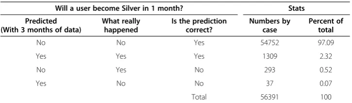
Table 8 Precision and accuracy of silver attainment
Will a user become Silver in 1 month? Stats
Predicted (With 3 months of data)
What really happened
Is the prediction correct?
Numbers by case
Percent of total
No No Yes 54752 97.09
Yes Yes Yes 1309 2.32
No Yes No 293 0.52
Yes No No 37 0.07
Total 56391 100
Notes: Prediction performed for each passenger with 3 month of data since 1st flight at time point: end of the three months. Precision = 2.75%. Accuracy = 81.71%.
Table 7 Comparison of prediction power of extrapolation vs. D/S model
Question asked D months after 1st flight: will they becomeSilverwithin S months? Case D S Extrapolation of miles Rx1 D/S Model Rx2P3A4
0 0.5 3 0.39 0.60 81% 31%
1 1 1 0.39 0.71 87% 53%
2 1 2 0.39 0.70 89% 48%
3 3 1 0.50 0.89 97% 82%5
4 3 3 0.39 0.67 95% 46%
5 6 3 0.51 0.83 96% 69%
Notes.1
To compare predictive power between two models we use correlation as a proxy. Rx = correlation of accumulated miles with binary variable silver_attain.2correlation of the Model’s prediction with binary variable silver_attain.3
P = Precision, of all users who were predicted to become Silver, How many of them did indeed become silver?4
100% with no false positives for both models. After this proof the company was con-vinced about the validity of the model and asked us to provide code to integrate it with his existing CRM system.
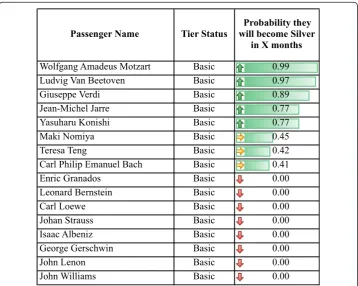
How can this knowledge help to create value? Let’s consider a flight from ADX to TYO. There are only five available seats in business class. Let’s assume that these five seats can be used to upgrade five lucky passengers. Of the 150 passengers expected to board the flight, lets assume that 20 are eligible for upgrade. The model will take less than one second to rank all the 150 passengers by probability of becoming Silver. Most importantly, it will also rank the 20 candidates. Figure 4 shows an example app. With this ranking at hand, we can now rationally allocate the five upgrades to the five customers most likely to become Silver rather than to customers with a zero probability of becoming Silver.
Discussion
By translating passenger data from“Airline”timeline to a timeline relative to each passenger first flight, we have shown that a D/S model yields high accuracies. Furthermore, taking ad-vantage of recently made available data mining libraries [9,10] we outperformed simple ex-trapolation models and previous works [5]. False positive rates are less than 3%. The causes of a false positive have not been investigated in the scope of this project, but can be due to either/or a combination of: (1) the predictive nature of the data is not unlimited. (2) The predictive power of the model can be improved. However, the most interesting result is that
the perceived value of a miles program can be increased dramatically to the very customers that matter most to the airline: the ones with high likelihood of becoming Silver.
In our experience with previous data mining projects, rather than fine tune models, the most effective way to improve accuracy is to add new features which are as uncor-related as possible with existing features. A good place to look for potential candidates are features derived from different data sources other than the Airline CRM database, for example publicly available social media data.
Competing interests
We do not have any competing interest. We do not work for any airline or have a commercial relationship with any airline or any financial interest.
Authors’contributions
JB developed de business logic and DE carried out the data modelling. All authors read and approved the final manuscript.
Acknowledgments
Sajat Kamal for the Aeroplan insights. Dr. Barry Green and Roy Kinnear showing themselves to be greater than their prejudices and letting us modelling the data.
Author details
1UAE University, 17551 Al Ain, Abu Dhabi, UAE.2Moscow State University, Leninskie gori 1, 117234, Moscow.
Received: 30 October 2013 Accepted: 20 February 2014 Published: 24 June 2014
References
1. Lawrence RD, Hong SJ, Cherrier J (2003) Passenger-based predictive modeling of airline no-show rates. Proceed-ings of the ninth SIGKDD international conference on Knowledge discovery and data mining. pp 397–406 2. Alaska Airlines GE Flight Quest data mining challenge 2013, http://www.gequest.com/c/flight
3. Liou JJH, Tzeng G-H (2010) A dominance-based rough set approach to customer behavior in the airline market. Inf Sci 180(11):2230–2238
4. Pritscher L, Feyen H (2001) Data mining and strategic marketing in the airline industry. Data Mining for Marketing Applications. Citeseer: http://citeseerx.ist.psu.edu/viewdoc/summary?doi=10.1.1.124.7062.
5. Malthouse EC, Blattberg RC (2005) Journal of Interactive Marketing. Can we predict customer lifetime value? Wiley Online Library: http://www.researchgate.net/publication/227633642_Can_we_predict_customer_lifetime_value/ file/60b7d517fd5bb2905e.pdf.
6. Aeroplan loyalty program, http://en.wikipedia.org/wiki/Aeroplan
7. Smith BC, Leimkuhler JF, Darrow RM (1992) Yield management at American airlines. Interfaces 22(1):8–31 8. Burges CJ (1998) A tutorial on support vector machines for pattern recognition. Data Min Knowl Disc 2(2):121–167 9. (2013) Greg Ridgeway with contributions from others. gbm: Generalized Boosted Regression Models. R package
version 2.0-8. http://CRAN.R-project.org/package=gbm
10. Ian M (2012) glm2: Fitting Generalized Linear Models. R package version 1.1.1. http://CRAN.R-project.org/ package=glm2
11. Valentini G, Masulli F (2002) Ensembles of learning machines. Neural Nets. Springer, Berlin Heidelberg, pp 3–20
doi:10.1186/2196-1115-1-3
Cite this article as:Berengueres and Efimov:Airline new customer tier level forecasting for real-time resource allocation of a miles program.Journal of Big Data20141:3.
Submit your manuscript to a
journal and benefi t from:
7Convenient online submission
7Rigorous peer review
7Immediate publication on acceptance
7Open access: articles freely available online
7High visibility within the fi eld
7Retaining the copyright to your article