SmartTracing: self-learning-based Neuron reconstruction
Hanbo Chen•Hang Xiao•Tianming Liu•Hanchuan Peng
Received: 3 July 2015 / Accepted: 4 August 2015 / Published online: 19 August 2015 ÓThe Author(s) 2015. This article is published with open access at Springerlink.com
Abstract In this work, we propose SmartTracing, an automatic tracing framework that does not require sub-stantial human intervention. There are two major novelties in SmartTracing. First, given an input image, SmartTracing invokes a user-provided existing neuron tracing method to produce an initial neuron reconstruction, from which the likelihood of every neuron reconstruction unit is estimated. This likelihood serves as a confidence score to identify reliable regions in a neuron reconstruction. With this score, SmartTracing automatically identifies reliable portions of a neuron reconstruction generated by some existing neuron tracing algorithms, without human intervention. These reliable regions are used as training exemplars. Second, from the training exemplars the most characteristic wavelet features are automatically selected and used in a machine learning framework to predict all image areas that most probably contain neuron signal. Since the training samples and their most characterizing features are selected from
each individual image, the whole process is automatically adaptive to different images. Notably, SmartTracing can improve the performance of an existing automatic tracing method. In our experiment, with SmartTracing we have successfully reconstructed complete neuron morphology of 120Drosophilaneurons. In the future, the performance of SmartTracing will be tested in the BigNeuron project (bigneuron.org). It may lead to more advanced tracing algorithms and increase the throughput of neuron mor-phology-related studies.
Keywords SmartTracingNeuron reconstruction
Neuron morphologyMachine learningReconstruction confidence
1 Introduction
The manual reconstruction of a neuron’s morphology has been in practice for one century now since the time of Ramo´n y Cajal. Today, the technique has evolved such that researchers can quantitatively trace neuron morphologies in 3D with the help of computers. As a quantitative description of neuron morphology, the digital representa-tion has been widely applied in the tasks of modern neu-roscience studies [1–3] such as characterizing and classifying neuron phenotype or modeling and simulating electrophysiology behavior of neurons. However, many popular neuron reconstruction tools such as Neurolucida (http://www.mbfbioscience.com/neurolucida) still rely on manual tracing to reconstruct neuron morphology, which limits the throughput of analyzing neuron morphology.
In the past decade, many efforts have been given to eliminate such a bottleneck by developing automatic or semi-automatic neuron reconstruction algorithms [1,3]. In H. Chen (&)H. Peng
Allen Institute for Brain Science, Seattle, WA, USA e-mail: [email protected]
H. Peng
e-mail: [email protected]
H. ChenT. Liu
Cortical Architecture Imaging and Discovery Lab, Department of Computer Science and Bioimaging Research Center, The University of Georgia, Athens, GA, USA
H. Xiao
CAS-MPG Partner Institute for Computational Biology, Shanghai Institutes for Biological Sciences, Chinese Academy of Sciences, 320 Yueyang Road, Shanghai, China
these algorithms, different strategies and models were applied, such as pruning of over-complete neuron trees [4, 5], shortest path graph [6], distance transforms [7], snake curve [8], and deformable curve [9]. However, the completeness and the attribute of resulted neuron mor-phology vary tremendously between different algorithms. Recently, to quantitatively assess such variability between algorithms and advance the state of the art of automatic neuron reconstruction method, a project named BigNeuron [10, 11] has been launched to bench-test existing algo-rithms on big dataset. One reason causing such variability is that image quality and attributes vary between different data sets—partially due to the differences in imaging modality, imaging parameter, animal model, neuron type, tissue processing protocol, and the proficiency of micro-scopic operator. And some of the algorithms were devel-oped based on specific data or were develdevel-oped to solve specific problem in the data which may not be applicable for other types of data. Another reason is that most of the tracing algorithms required user input of parameters. As a consequence, the optimal parameters vary between images and thus require manual tuning by the user with sufficient knowledge of the algorithm.
We note that most of the current automatic neuron reconstruction algorithms are not ‘‘smart’’ enough. Indeed, many times they require human intervention to obtain reasonable result. To conquer this limitation, one can adapt learning-based methods; so the algorithm can be trained for different data. In [12], the authors proposed a machine learning approach to estimate the optimal solution of linking neuron fragments. However, the fragments to link were still generated by model-driven approaches, and it requires manual work in generating training samples.
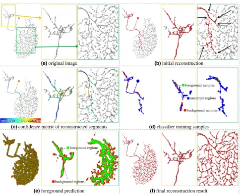
In this paper, based on machine learning algorithms, we proposed SmartTracing, an automatic tracing framework that does not require human intervention. The procedure of the SmartTracing algorithm is outlined in Fig.1. First, the initial reconstruction was obtained based on existing automatic tracing algorithms (Fig.1b). Second, a confi-dence metric proposed in this paper was computed for each reconstruction segment to identify reliable tracing (Fig.1c). Third, a training sampler (Fig.1d) and the most characteristic features were obtained. Fourth, a classifier was then trained and the foreground containing neuron morphology was predicted (Fig.1e). Finally, after adjust-ing the image based on prediction result, the final recon-struction was traced (Fig.1f).
The paper is organized as follows. We first discuss the key steps of SmartTracing. Then we describe the imple-mentation and the availability of the algorithm. Finally, we present experimental results on real neuron image data, followed by some brief discussion of the pros and cons and the future extension of SmartTracing.
2 Method
2.1 Automatic search training exemplars
2.1.1 Confidence score of reconstruction
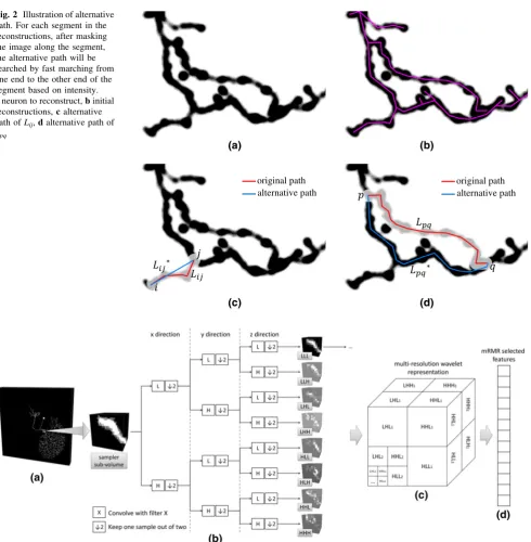
In SmartTracing, we first identify the reliable neuron reconstructions as training exemplars. A neuron recon-struction can be decomposed into multiple segments by breaking the reconstruction at the branch point. Whether or not a segment is trustworthy can be tested by checking if there is an alternative path connecting the two ends of the segment compared to this segment. Our premise is that a segment with no better alternative pathway (e.g., Fig-ure2c) is more reliable in comparison with a segment with alternative pathway (e.g., Figure2d). Specifically, for a segment Lij between points i and j, the image intensity
alongLijwill be masked to 0 first. Then, the shortest path
Lij weighted by intensity between points i and j will be
identified. In the original image, the average intensity along Lij andLijwill be measured:
Iij¼ R
LijIðxÞdx
Lij ; ð1Þ
whereI(x) is the intensity ofxandLijis the length ofLij.
Then the confidence metric can be obtained by dividing Iij
byIij:
Cij¼Iij=Iij: ð2Þ
Our method is that if an alternative path exists,Iij will be closer to or even larger thanIijandCijwill be close to 1.
Otherwise, Lij will be a relatively straight line passing through background with low intensity connectingiandj, and thus Cij1. This measurement is based on the assumption that background intensity is lower than fore-ground intensity. When the backfore-ground intensity is greater than foreground (e.g., for brightfield images), we can simply invertCijin Eq. (2).
2.1.2 Obtaining training exemplars
are taken as uncertain regions as well. These 3 types of regions compose 3 layers surrounding the confident recon-structions—core layer: foreground samples; middle layer: uncertain regions; and outer layer: background samples.
2.2 Extracting features for classification
Image intensity-based features are extracted by adopting the method proposed in [13]. The whole procedure is outlined in Fig.3. For each sample voxel, features are extracted in a 3D cube surrounding this voxel (Fig.3a). Multi-resolution wavelet representation (MWR) is applied to project the sub-volume of the local 3D cube into a feature space (Fig.3b. c). Then, a subset of features is selected based on minimum-Redundancy Maximum-Rele-vance (mRMR) method [14] for classification (Fig.3d).
MWR codes the information in both frequency domain and spatial domain. It is effective for identifying local and multi-scale features from signals or images and has been widely used in pattern recognition tasks. The MWR framework was firstly introduced on 1-dimensional (1D) signals and then extended to 2-dimensional (2D) images by Mallat [15]. In brief, a pair of functions was defined to conduct wavelet transform—the mother wavelet w(x)— representing the detail and high-frequency parts of a signal and the scaling function u(x) representing the smooth and low-frequency parts of the signal. To decompose signal into multiple resolutions, the calculation is performed iteratively on the smoothed signal calculated based on u(x). In practice, for discrete signal, instead of calculating waveletw(x) and scaling functionu(x), a high pass filter H and a low pass filter L will be applied to calculate MWR.
(a) original image
(e) foreground prediction
(b) initial reconstruction
(d) classifier training samples
(f) final reconstruction result
confident not confident
foreground samples
foreground regions
background samples uncertain regions
background regions
(c) confidence metric of reconstructed segments
Fig. 1 Overview of SmartTracing method and the result for a single image. In each sub-figure, the global 3D view of images and the overlapped reconstructions is shown on theleft. The zoomed-in 3D
Mallat has shown that MWR can be extended from 1D signal to 2D image by convolving the image with the filters in one dimension first and then convolving the output image with the filters in the other dimension [15]. Such operation can be further extended to 3D volume [16]. As illustrated in Fig.3b, in one level of decomposition, 8 groups of wavelet coefficients are obtained by convolving volume with different permutations of two filters in three
directions successively. The smoothed volume LLL is further decomposed in the next level to achieve multi-resolution representations.
After MWR decomposition, the dimension of feature space is relatively high—the number of featuresffigequals the number of voxels in the sub-volume (Fig.3c). Since some of these features may carry redundant information or non-discriminative information, using the full set of MWR
Fig. 3 Illustration of feature selection procedure.aExtracting sub-volume in 3D cube surrounding the sample voxel.bWavelet decomposition for volume data.cMulti-resolution wavelet representation.dSelecting a characterizing subset of features based on mRMR for classification
(b) (a)
(c) (d)
∗ ∗
alternative path original path
alternative path original path Fig. 2 Illustration of alternative
path. For each segment in the reconstructions, after masking the image along the segment, the alternative path will be searched by fast marching from one end to the other end of the segment based on intensity.
aneuron to reconstruct,binitial reconstructions,calternative path ofLij,dalternative path of
coefficients directly may lead to inaccurate result. To better discriminate patterns and improve the robustness and accuracy of training framework, we select the most char-acterizing subset of features S. We consider the mRMR feature selection method to solve the problem. The algo-rithm has been widely applied in selecting features in high-dimensional data such as microarray gene expression data to solve classification problems [17]. In the algorithm, the statistical dependency between the exemplar type and the joint distribution of the selected features will be maxi-mized. To meet this criterion, mRMR method search for the features that are mutually far away from each other (minimum redundancy) but also individually most similar to the distribution of sampler types (maximum relevance). In practice, these two conditions were optimized simultaneously:
max S2W
1 S j j
X
i2S
Iðc;fiÞ 1 S j j2
X
i;j2S Iðfi;fjÞ
( )
; ð3Þ
where W denotes the full set of MWR coefficients, c denotes the vector of sampler type, j jS is the number of features, and I(x, y) is the mutual information between x andy. The first term in the equation is the maximum rel-evance condition, and the second term is the minimum redundancy condition. It has been shown in [14] that the solution can be computed efficiently inOðj j S j jÞW .
2.3 Training classifier and tracing neuron reconstruction
Based on the extracted features of training samplers, supervised training can be performed to train a classifier for foreground/background predictions. In our proposed framework, we use Support Vector Machine (SVM) implemented in LIBSVM tool kit [18]. The default parameter setting of LIBSVM is used. A subset of fore-ground and backfore-ground training samplers is randomly chosen from the pool to make sure that the numbers of training samplers from each class are the same.
With the trained classifier, we then examine the voxels in the image and label them as foreground or background (Fig.1e). Since in neuron tracing problem foreground signals are often sparse and relatively continuous in the image, we use a fast marching algorithm to search for the foreground signals. Initially, the voxels of foreground samples are pre-labeled as foreground and the rest voxels are marked ‘‘unknown.’’ The algorithm would then march from foreground voxels to their adjacent unknown voxels. For each of such ‘‘unknown’’ voxels, its feature will be extracted and will be classified into foreground or back-ground based on the classifier trained. If the voxel is
classified as foreground, it will be taken as a new starting point for the next round of marching. The marching will stop if no more foreground voxel can be reached, and all of the unknown voxels left will be labeled as background.
Based on the labeled image, the original image is adjusted to obtain the final tracing result. The intensity of background voxels is set to 0. For foreground voxel, if its intensity is lower than threshold set for tracing algorithm, the intensity of the voxel will be set as the threshold value. Otherwise, its intensity will be kept unchanged. Then the tracing algorithm will be re-run on the adjusted image to trace the final corrected neuron reconstruction.
3 Implementation
4 Experimental results
The whole framework was tested on 120 confocal images of single neurons in theDrosophilabrain downloaded from the flycircuit.tw database. The dimension of each image is 1024910249120 voxels. For some of the images, APP2 works reasonably well in reconstructing neuron mor-phologies. However, due to the loss of signals during image preprocessing, there could be a gap between neuron segments which resulted in incomplete reconstructions by
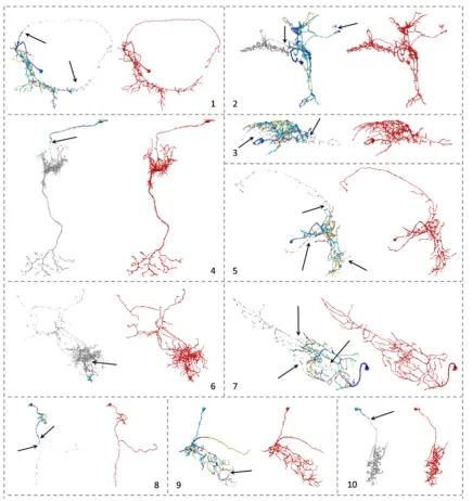
APP2. Ten examples of incomplete reconstructions were shown and highlighted by arrows in Fig.4. Those gaps were classified as foreground with proposed SmartTracing framework and filled for complete tracing (red skeletons in Fig.4). The quantitative measurements of the morphology and the computational running time (using single CPU) of these 10 examples are listed in Table 1.
For the 120 confocal images tested, the proposed SmartTracing algorithm successfully improved the overall completeness of reconstructions. In comparison with initial
Fig. 4 Visualization of reconstructed neuron morphology of 10
selected examples. In each sub-figure, initial reconstruction generated by APP2 (coloredskeletons) was overlapped on the original image (grayskeletons). The corresponding final reconstruction obtained by SmartTracing was shown inredskeletons on the right. The initial
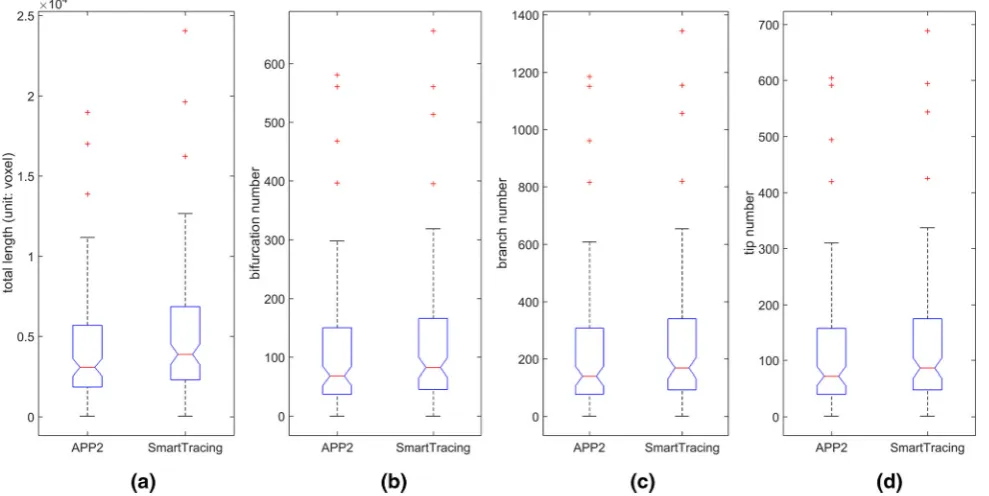
reconstructions, the total length, bifurcation number, branch number, and tip number all increased after the optimization of SmartTracing (Fig.5). Among those, the completeness of 30 reconstructions was significantly improved (the total length of final reconstruction is 1.2 times larger than that of initial reconstruction). By visual inspection, the SmartTracing algorithm only failed to trace the complete neuron morphology on 1 image out of the 120
images. In this failure case, there is a gap that is too big to be filled (Fig.6b).
Notably, SmartTracing is able to run iteratively. The reconstruction generated from the previous round is used as the initial reconstruction for the next round. However, for the reconstruction that is relatively complete, further iter-ation will not change the result significantly (Fig. 6a) and is time consuming. On the other hand, for the incorrect
Table 1 The running time of each procedure and the quantitative neuron morphology measurement of 10 selected example datasets
ID Running time (seconds) Length Bifurcation Branch Tip
Tin Ts Tm Tt Tp Tst Rin Rst Rin Rst Rin Rst Rin Rst
1 10.4 254 0.19 12.7 110 12.7 3027 4686 69 74 141 153 72 79
2 10.6 456 0.22 17.9 185 15.1 4469 7557 112 180 228 367 116 187
3 11.1 474 0.23 12.1 89 14.6 4611 6163 145 159 293 325 149 167
4 9.2 310 0.17 7.4 58 15.9 483 5823 5 117 11 240 7 124
5 10.9 310 0.19 8.5 119 16.7 3992 5635 84 92 175 188 91 96
6 9.2 29 0.17 7.5 133 22.2 176 8298 4 174 9 359 6 186
7 9.3 249 0.16 7.9 120 19.2 4408 7016 74 98 151 198 77 101
8 9.3 61 0.17 11.6 69 9.9 545 1174 7 8 14 16 8 9
9 10.1 307 0.17 9.2 53 13.4 3021 4024 75 93 155 190 81 98
10 9.0 37 0.16 7.3 78 15.3 125 3494 2 76 5 159 3 83
Visualization of the morphology of reconstructions and the original image of these examples are shown in Fig.4
Tingenerating initial reconstruction by APP2; Tscomputing confidence score; TmmRMR feature selection; TtSVM classifier training; Tp searching foreground;Tstgenerating final reconstruction;Rininitial reconstruction;Rstfinal reconstruction;Length unit: voxel
Fig. 6 Examples of performing SmartTracing iteratively. Recon-struction shown inredtube is overlapped on the original image shown in gray. a Reconstruction of the first and second rounds of SmartTracing of case #7 shown in Fig.4. bReconstruction of the
case that failed in the first round of SmartTracing but succeeded after tworoundsshown in different angles. The gap that caused the failure in the first round ishighlightedbyarrows. (Color figure online)
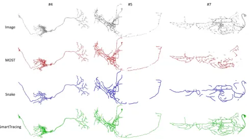
Fig. 7 Comparisons of the reconstructions generated by 3 different tracing algorithms using 3 testing images. Image ID is the same as Fig.4. The original images are shown in thetop rowfollowed by the
reconstruction, better training samples could be obtained based on the reconstruction from the previous iteration which may successively remedy the reconstruction. Thus we tried performing SmartTracing iteratively on the pre-viously failed case. Intriguingly, it only took two rounds of SmartTracing to successfully fill the gap and obtain com-plete reconstruction (Fig.6b). This is mainly because. with the result from the first round, more training samples from the gap area were obtained to train the classifier, so the gap can be filled in the second round.
We then compared the result generated by SmartTracing with other methods. Specifically, the results generated by micro-optical sectioning tomography (MOST) ray-shooting tracing [21] and open-curve snake (Snake) tracing [8,22] were compared. By visual inspection, the results generated by our proposed SmartTracing were more complete, more topologically correct, and better at reflecting the mor-phology of the neurons in original images than other tracing methods (Fig.7).
5 Discussion
In our experiments, the proposed SmartTracing method improved the APP2 tracing and successfully reconstructed 120Drosophilaneurons from confocal images. In addition to filling the gaps between neuron segments, SmartTracing can also reduce over-traces due to image noise, inhomo-geneous distribution of image intensity, and inappropriate tracing parameters. Essentially, SmartTracing is an adap-tive and self-training image preprocessing procedure that segments the image into the foreground area containing neuron signals and the background voxels. The major novelty of SmartTracing lies in two aspects.
First, we proposed a likelihood measurement that serves as a confidence score to identify reliable regions in a neuron reconstruction. With this score, reliable portions of a neuron reconstruction generated by some existing neuron tracing algorithms are identified, without human intervention, as training exemplars for learning-based tracing method. On the other hand, the human proof-reader can also benefit from the metric. By ranking the reconstructions by the confidence score, the human annotators are able to prioritize on the less-reliable reconstructions, which increases the overall accuracy and saves time.
Second, from the training exemplars the most charac-teristic wavelet features are automatically selected and used in a machine learning framework to predict all image areas that most probably contain neuron signal. Since the training samples and their most characterizing features are selected from each individual image, the whole process is auto-matically adaptive to different images and does not require
prior knowledge on the object to identify. Potentially, the proposed machine learning and prediction framework can be extended to other image segmentation tasks and 3D object recognition systems such as neuron spine detection, cell segmentation, etc.
SmartTracing is applicable to most of the existing tracing algorithms. However, the performance and the outcome of SmartTracing largely relied on the tracing algorithm applied. For instance, the cause of the only failed case among 120 tested images is that APP2 did not gen-erate sufficient initial reconstruction due to the gap which results in a lack of training exemplars. One solution to this limitation is to run SmartTracing iteratively, so better training samples can be acquired from the previous itera-tion. Also, we can take the merit of different tracing algorithms and use different algorithms in different steps to further improve the performance of the framework—e.g., use MOST algorithm to generate initial tracing for scoring and thus training since it is not sensitive to gaps and can capture more signals; then use APP2 to generate final tracing since it is robust, efficient, and optimal to generate tree shape topology of neurons.
Another limitation of SmartTracing is the relatively high computational complexity. At present, the top two time-consuming procedures are the computation of confidence metric, which is proportional to the initial neuron recon-struction complexity, and the predictions of foreground voxels, which is proportional to the size of the neuron. The previously reported computation time is calculated based on a single CPU. With parallel computation framework, both steps can be sped up.
In recent years, a growing number of model-driven approaches have been proposed for automatic neuron reconstructions. To our best knowledge, SmartTracing is one of the earliest machine learning-based methods for automatic neuron reconstruction. Different from the tra-ditional learning-based method, SmartTracing does not require human input of training exemplars and can self-adapt to different types of neuroimage data. Additionally, the method can be applied to improve the performance of other existing tracing methods. As part of future work, the performance of SmartTracing will be further exam-ined and improved by BigNeuron project. In the near future, we hope that SmartTracing can significantly facilitate manual tracing and contribute to the neuron morphology reconstructions in large.
References
1. Donohue DE, Ascoli GA (2011) Automated reconstruction of neuronal morphology: an overview. Brain Res Rev 67:94–102 2. Parekh R, Ascoli GA (2013) Neuronal morphology goes digital: a
research hub for cellular and system neuroscience. Neuron 77:1017–1038
3. Meijering E (2010) Neuron tracing in perspective. Cytometry A 77:693–704
4. Xiao H, Peng H (2013) APP2: automatic tracing of 3D neuron morphology based on hierarchical pruning of a gray-weighted image distance-tree. Bioinformatics 29:1448–1454
5. Peng H, Long F, Myers G (2011) Automatic 3D neuron tracing using all-path pruning. Bioinformatics 27:i239–i247
6. Lee P-C, Chuang C-C, Chiang A-S, Ching Y-T (2012) High-throughput computer method for 3D neuronal structure recon-struction from the image stack of the Drosophila brain and its applications. PLoS Comput Biol 8:e1002658
7. Yang J, Gonzalez-Bellido PT, Peng H (2013) A distance-field based automatic neuron tracing method. BMC Bioinform 14:93 8. Wang Y, Narayanaswamy A, Tsai C-L, Roysam B (2011) A
broadly applicable 3-D neuron tracing method based on open-curve snake. Neuroinformatics 9:193–217
9. Peng H, Ruan Z, Atasoy D, Sternson S (2010) Automatic reconstruction of 3D neuron structures using a graph-augmented deformable model. Bioinformatics 26:i38–i46
10. Peng H, Meijering E, Ascoli GA (2015) From DIADEM to BigNeuron. Neuroinformatics 13:259–260
11. Peng H, Hawrylycz M, Roskams J, Hill S, Spruston N, Meijering E, Ascoli GA (2015) BigNeuron: large-Scale 3D neuron recon-struction from optical microscopy images. Neuron. doi:10.1016/j. neuron.2015.06.036
12. Gala R, Chapeton J, Jitesh J, Bhavsar C, Stepanyants A (2014) Active learning of neuron morphology for accurate automated tracing of neurites. Front Neuroanat 8:37
13. Zhou J, Peng H (2007) Automatic recognition and annotation of gene expression patterns of fly embryos. Bioinformatics 23:589–596
14. Peng H, Long F, Ding C (2005) Feature selection based on mutual information: criteria of max-dependency, max-relevance, and min-redundancy. IEEE Trans Pattern Anal Mach Intell 27:1226–1238
15. Mallat SG (1989) A theory for multiresolution signal decompo-sition: the wavelet representation. IEEE Trans Pattern Anal Mach Intell 11:674–693
16. Muraki S (1993) Volume data and wavelet transforms. IEEE Comput Graph Appl 13:50–56
17. Ding C, Peng H (2005) Minimum redundancy feature selection from microarray gene expression data. J Bioinform Comput Biol 3:185–205
18. Chang C-C, Lin C-J (2011) LIBSVM: a library for support vector machines. ACM Trans Intell Syst Technol 2:1–27
19. Peng H, Ruan Z, Long F, Simpson JH, Myers EW (2010) V3D enables real-time 3D visualization and quantitative analysis of large-scale biological image data sets. Nat Biotechnol 28:348–353
20. Peng H, Bria A, Zhou Z, Iannello G, Long F (2014) Extensible visualization and analysis for multidimensional images using Vaa3D. Nat Protoc 9:193–208
21. Wu J, He Y, Yang Z, Guo C, Luo Q, Zhou W, Chen S, Li A, Xiong B, Jiang T, Gong H (2014) 3D BrainCV: simultaneous visualization and analysis of cells and capillaries in a whole mouse brain with one-micron voxel resolution. Neuroimage 87:199–208
22. Narayanaswamy A, Wang Y, Roysam B (2011) 3-D image pre-processing algorithms for improved automated tracing of neu-ronal arbors. Neuroinformatics 9:219–231
Hanbo Chenis pursuing his Ph.D. degree in computer science at The University of Georgia. His research interest lies in studying brain network and developing method for high-dimensional big data analysis which includes multi-scale, multi-modal, multi-subject, and across species brain image data.
Hang Xiao received the B.S. degree in Biology from Wuhan
University in 2008 and the Ph.D degree in Computational Biology from CAS-MPG Partner Institute in 2014. He visited Janelia Farm Research Campus between 2011 and 2012. His current interest includes pattern recognition, deep learning, and neuron tracing methods.
Tianming Liuis a Professor of Computer Science at The University of Georgia. His research area is brain mapping, and he has published over 160 peer-reviewed articles in this area. Dr. Liu is the recipient of both NSF CAREER award and NIH Career award in the area of brain imaging and mapping.
Hanchuan Pengleads a group of computational neuroanatomy and