R E G U L A R A R T I C L E
Open Access
Testing Heaps’ law for cities using
administrative and gridded population data
sets
Filippo Simini
1*and Charlotte James
1*Correspondence: [email protected] 1Department of Engineering
Mathematics, University of Bristol, Bristol, UK
Abstract
Since 2008 the number of individuals living in urban areas has surpassed that of rural areas and in the next decades urbanisation is expected to further increase, especially in developing countries. A country’s urbanisation depends both on the distribution of city sizes, describing the fraction of cities with a given population (or area), and the overall number of cities in the country. Here we present empirical evidence suggesting the validity of Heaps’ law for cities: the expected number of cities in a country is only a function of the country’s total population (or built-up area) and the distribution of city sizes. This implies the absence of correlations in the spatial distribution of cities. We show that this result holds at the country scale using the official administrative definition of cities provided by the Geonames dataset, as well as at the local scale, for areas of 128×128 km2in the United States, using a morphological definition of urban clusters obtained from the Global Rural-Urban Mapping Project (GRUMP) dataset. We also derive a general theoretical result applicable to all systems characterised by a Zipf distribution of group sizes, which describes the relationship between the expected number of groups (cities) and the total number of elements in all groups (population), providing further insights on the relationship between Zipf’s law and Heaps’ law for finite-size systems.
Keywords: Heaps’ law; Zipf’s law; Cities; Urbanisation; Scaling
1 Introduction
The increase of urbanisation rates, generally defined as the increase of the proportion of people living in urban areas or the proportion of buildings belonging to urban agglomera-tions [1], is a trend that has happened in waves throughout human history, with a dramatic acceleration in the last 300 years [2]. In 2015, 56% of China’s population lived in cities, a fig-ure that has more than doubled compared to 26% of 1990. The Ministry of Housing and Urban-Rural Development estimates that by 2025 300M Chinese now living in rural areas will move into cities. State spending is planned on new houses, roads, hospitals, schools, which could cost up to 600 billion US dollars a year. A great rate of urbanisation is also expected in Sub-Saharan African countries. As a result, by 2030 it is estimated that the world’s population will have increased by over 1 billion people most of whom will dwell in the rapidly growing cities of Asia and Africa [3]. Recent studies show that, on average,
urban land is expanding at twice the urban population growth rate, resulting in a decrease of urban population density with time [4].
A quantitative understanding of the mechanisms that drive urbanisation is important for helping governments and decision makers to plan investments in order to achieve sus-tainable urban planning and growth. These decisions will have a huge impact on the lives of millions of people, the economy and the environment. Urbanisation can happen in two ways: diffusion (or sprawl) and aggregation. Diffusion corresponds to existing cities grow-ing and increasgrow-ing in size because of either net migration from rural areas or a greater rate of natural increase (i.e. birth rate minus death rate) in urban areas. Aggregation cor-responds to new villages and towns being created in rural areas that were previously con-sidered non-urbanised. In order to properly characterise urbanisation patterns we should consider both aspects: the distribution of city sizes, describing the size and growth of ex-isting cities, and the overall number of cities, describing the abundance and formation of new urban areas.
The distribution of city sizes is a broad and heterogeneous distribution. Ranking cities by population, it has been observed [5–7] that the population of thei-th largest city of a country is approximately equal to the population of the largest city divided byi, i.e. a city’s rank is inversely proportional to its population. In other words, the fraction of cities with population larger thanxfollows Zipf ’s law,P(>x)∼x–α, withα1. Previous studies have
shown how Zipf ’s law can originate from various models based on cluster growth and ag-gregation [8–11], the interplay between multiplication and diffusion processes [12], pref-erential migration to large aggregates [13], pairwise interactions between individuals [14] and proportionate random growth [15–17], or Gibrat’s law [18,19].
Compared to the great efforts made to characterise the distribution of city sizes both empirically and theoretically, much less work has been done to answer the other funda-mental question about the urbanisation process: What determines the number of cities in a country? In this paper we empirically investigate the relationships between the number of cities in a region and some of the region’s properties, such as the region’s total popu-lation and built-up area. In particular, we consider how the total popupopu-lation (or the total built-up area) of a region affects the number of cities. This is analogous to Heaps’ Law in linguistics [20,21], which describes the empirical scaling relationship between the num-ber of distinct words,W, in a document and the total number of words in the document (or text length),N:W∼Nγ, whereγ ≤1 is the Heaps exponent.
Previous research has shown that Zipf ’s law and Heaps’ law often appear together, sug-gesting that the presence of Zipf ’s law implies Heaps’ law. Considering the probability density function (PDF) corresponding to Zipf ’s Law,P(x)∼x–1–α, it can be shown [22]
and still be a power-law, but the size distributions in the regions would not follow Zipf ’s law anymore and as a consequence Heaps’ law would not hold. Indeed, this is what happens in ecological systems, where macro-ecological statistical patterns of species distribution and abundance display a strong dependence on the spatial scale considered [23]. One of the most relevant statistics used to characterise the degree of biodiversity of ecosystems is the species-area relationship (SAR), which measures the number of different species expected to be found in areas of increasing size. Since the density of individuals per unit area is constant, the SAR is the equivalent of Heaps’ law for ecosystems, as it measures the relationship between a region’s total population and the expected number of differ-ent groups of individuals in the region, where here groups correspond to species instead of cities. Empirical measurements of the SAR show a different functional behaviour as the region’s area increases, and this is due to the fact that the shape of the distribution of species sizes, called the relative species abundance, depends on the spatial scale consid-ered. While there are various studies on Heaps’ law in linguistics and SAR in ecology, to the best of our knowledge there is no thorough empirical analysis of Heaps’ law in urban systems. The aim of this paper is to precisely fill this gap and to investigate the validity of Heaps’ laws for cities.
There is another reason to investigate the relationship between Zipf ’s and Heaps’ laws for cities. Zipf ’s law for the distribution of city sizes usually holds only for the tail of the distribution, however the fact that in a region the distribution of city sizes has a power-law tail does not give any information regarding the relationship between the number of cities in the region and its total population. In other words, when Zipf ’s law holds only for large cities, there is no guarantee that Heaps’ law holds as well. To understand this, consider a region in which city sizes follow Zipf ’s law. If the population of each city is doubled and hence the total population of the region is also doubled, yet no new cities are created, Zipf ’s law will still be present, albeit with a larger scale parameter (i.e. the minimum city size is doubled). However, Heaps’ law will not hold in this case, because the total population,N, is doubled, but the number of cities,C, has not changed.
In this paper, we use a dataset on the population and location of cities globally to as-sess if Heaps’ law holds for all countries in all continents (except Australia and Antartica), and to test the predicted relationship between Heaps’ and Zipf ’s exponents. Cities can be defined in many different ways and various relevant properties of urban agglomerations, including the scaling relationships between population size and urban indicators such as area of roads and number of patents, depend on the method used to define cities [24,25]. In particular, the relationship between the number of cities in a region and the region’s total population, i.e. Heaps’ law, can also depend on the definition of city considered. To understand how Heaps’ law depend on the definition of city, we use a second dataset of the spatial distribution of population in the United States that allows us to consider various definitions of urban clusters and provide additional support to our results.
2 Analytical results
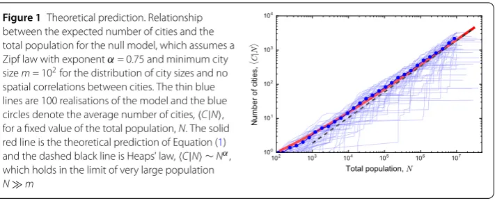
Figure 1Theoretical prediction. Relationship between the expected number of cities and the total population for the null model, which assumes a Zipf law with exponentα= 0.75 and minimum city sizem= 102for the distribution of city sizes and no spatial correlations between cities. The thin blue lines are 100 realisations of the model and the blue circles denote the average number of cities,C|N, for a fixed value of the total population,N. The solid red line is the theoretical prediction of Equation (1) and the dashed black line is Heaps’ law,C|N ∼Nα, which holds in the limit of very large population
Nm
One realisation of the model consists in drawing cities from this global distribution until a given target total size of the region,N, is reached. As soon as the sum of the city sizes becomes larger thanNthe drawing stops and the number of cities,C, corresponds to the number of drawings in this realisation. Repeating this process and averaging over many realisations it is possible to estimate the expected number of cities for a fixed target total populationN,C|N. VaryingN, one can study the dependence of the expected number of cities on the region’s total population and assess the validity of Heaps’ law.
A simple calculation shows that, under the assumptions of this null model, Heaps’ law holds asymptotically for very large populations, as reported in the literature [22]. Addi-tionally, our calculation allows us to derive a more accurate formula for the relationship between the number of cities and the total population, which is valid for smaller popula-tions as well. Let us consider the probability to find a city with populationxwithin a group ofCcities with total populationN,p(x|C,N). We can use this probability to compute the average population of such a group of cities, which is equal to N/C: N=C· x|C,N, wherex|C,Ndenotes the conditional expectation ofxgivenCandN. Multiplying by the probability to findCcities in a region with total populationN,p(C|N), on both sides and integrating with respect toCwe getN= dCp(C|N)C dxxp(x|C,N). If the prob-abilityp(x|C,N) can be considered independent of the number of cities whenC1, i.e.
p(x|C,N)≈p(x|N) and thusx|C,N ≈ x|N, then the expected number of cities in a re-gion with populationNisC|N ≈N/x|N. Using the assumption that city sizes follow Zipf ’s law with exponentα< 1 and given that the maximum city size cannot be larger than the region’s total population, we can writep(x|N) =α/(m–α–N–α)x–1–α(N–x), where mis the minimum city size andis the Heaviside step function. From this, we obtain the following equation relating the average number of cities and the total population:
C|N ≈1 –α
α ·N
(m–α–N–α)
(N1–α–m1–α), (1)
wheremrepresents the minimum city size. Note thatC|Nis a function of the ratioN/m. When the region’s population is very large,Nm, Equation (1) can be approximated as
C|N ∼(N/m)α, i.e. we obtain Heaps’ law. Figure1 shows 100 realisations of the null
model and the theoretical prediction given by Equation (1) forα= 0.75.
3 Heaps’ law for countries
Figure 2Heaps’ law for countries. (a), Zipf’s Law: PDF (y-axis) of city sizesX(x-axis) for all cities in Europe, America, Asia and Africa. The darker regions correspond to cities with populationX> 105, above which the distributions are a power law with exponentβ= 1 +αgiven in Table1. The dashed lines correspond to
y=x–β. Distributions have been shifted in they-axis for clarity.(b)–(c) and (e)–(f), Heaps’ law for America, Europe, Africa and Asia. The following information is displayed for each country: population (x-axis), number of cities with more than 100 k inhabitants (y-axis), logarithm of the area (marker size) and population density (color). The black line is a power law fit of the scaling relationship between the number of cities and the total population; Heaps exponentsγare reported in Table1. (d), The exponent of the Zipf PDF,β(y-axis) and the corresponding exponentγof Heaps’ law for Europe, America, Asia and Africa. Marker size corresponds to the minimum city population used in determining the values ofγandβ: values used are 103, 5×10³, 104and 105, where 103is represented by the smallest marker and 105by the largest. Increasing the minimum city population corresponds to a decrease in the amount of data used to fitγandβ: for a given continent, each point represents the same data set but restricted to a different range ofXvalues. The black dashed line corresponds to the relationship between the exponents,β=γ+ 1
country and the country’s total population. Since most countries have large populations, we expect that data should follow the asymptotic form of Heaps’ law,C∼Nα, if the
as-sumptions of our null model hold. To test this prediction, in Fig.2(a) we fit a power law to the tail of the empirical distribution of city sizes for each continent, obtaining the Zipf PDF exponentβ=α+ 1. Then we fit a power law to the scatter plot between the number of cities in each country and the country’s total population, Figs.2(b)–(c),2(e)–(f ), obtain-ing the Heaps exponentγ. Finally, we check if the value ofαis equal toγ for each of the continents, Fig.2(d).
The dataset used to perform this analysis is theGeonamesdataset [26], which consists of the population and geographic location of all cities with more than 1000 inhabitants worldwide. Data on the area and population of all countries was obtained from World-bank [27].
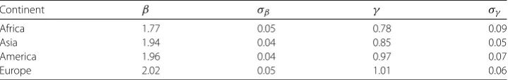
Table 1 Exponents of Zipf’s Law and Heaps’ Law. Column 1 displaysβ= 1 +α; the PDF exponent of Zipf’s Law with corresponding standard deviation displayed in column 2 for each of the four continents. Values were calculated by fitting a line to the PDF of city sizesXfor each continent, starting from a minimum population ofX= 105(see Fig.2(a)). Column 3 displaysγ; the exponent of Heaps’ Law with corresponding standard deviation displayed in column 4 for each of the four continents. Values ofγ and the error were obtained by fitting a line to the logarithm of Heaps’ Law; log(C) =γlog(N), for each continent (see Figs.2(b)–(c) and (e)–(f )). Exponentsβandγ were fit to the data using non-linear least squares
Continent β σβ γ σγ
Africa 1.77 0.05 0.78 0.09
Asia 1.94 0.04 0.85 0.05
America 1.96 0.04 0.97 0.07
Europe 2.02 0.05 1.01 0.06
Heap’s law We analyse the relationship between the number of cities in a country,C, and the country’s population,N, for all African, Asian, American and European countries (Fig.2(b)–(c) and (e)–(f )). We fit a power law to these data and obtain the Heaps exponents
γ reported in Table1. To test the validity of Heaps’ Law for cities, we assess the extent to which Heaps’ exponentsγare equal to the exponentsα=β– 1 from Zipf ’s Law. In Fig.2(d) we plotγ (x-axis) vsβ(y-axis) for different values of the minimum city population, where the exponents are fit to cities with population greater than this minimum population. The best fit values of Heaps exponentγ and Zipf PDF exponentβ=α+ 1 are compatible with the relationshipγ =αfor all the continents (see Table1), supporting the validity of the null model. The theoretical relationshipγ =β– 1 (black dashed line) is better satisfied when we consider large cities (> 105), whereas there are significant deviations for small values of minimum population. This is explained by the fact that the distributions of city sizes are not pure power laws, but there are deviations from Zipf ’s law for small cities (see Fig.2(a)).
Heaps’ law in the United States Heaps’ law is further confirmed by considering more homogeneous sets of regions, like the United States in Fig.3(a). There is clear evidence that the number of cities grows proportionally with the state population, whilst there is a small or indirect relationship between the number of cities and the state’s area or population density: in the United States, the cities-population, cities-area, cities-density correlation coefficients are 0.95, 0.04, and –0.08 respectively. In Fig.3(b) we plot the number of cities with more thanXinhabitants in each United States state,C(N,X), as a function of the ratioN/Xfor values ofXranging from 5000 to 5,000,000 inhabitants. All points collapse on a straight line, confirming that the equationC(N,X)∼N/Xholds for several orders of magnitude ofNandX. This is confirmed for the four continents as well (see see Additional file1). We also find evidence of the validity of Heaps’ law throughout time in the state of Iowa, United States. Historical data shows that between 1850 and 2000 the number of incorporated places (i.e. self-governing cities, towns, or villages) grew at the same rate as the state population (Fig.3(c)).
Figure 3Consequences of Heaps’ law. (a), The number of cities with more than 5000 inhabitants in the Unites States is proportional to the state’s population, corr(C,N) = 0.95. The correlations with area (0.04) and population density (–0.08, see inset) are negligible, as illustrated by the following pairs of states with similar area or density and very different number of cities: Alaska (A= 1.5M km2,C(5k) = 22) vs Texas (A= 0.7M km2,
C(5k) = 392), and Rhode Island (ρ= 393 km–2,C(5k) = 35) vs New Jersey (ρ= 467 km–2,C(5k) = 316). (b), Combining the result from panel (a) with Zipf’s law it is possible to estimate the number of cities with more thanXinhabitants in a country with populationNasC(N,X)∼N/X; Heaps’ law. As a consequence, the scattered cloud of points resulting when plottingC(N,X) againstNfor variousX’s in the range 5·103– 5·106 (inset) collapses on a straight line whenC(N,X) is plotted against the ratioN/X. (c), Historical records of the number of incorporated places (C, red triangles) and the state population (N, blue circles) in Iowa from 1850 to 2000 (source: State library of Iowa, state data center). The similar growth rates ofCandNentail the validity of Heaps’ lawC∼Nduring the 150-year period (inset). (d), The average distance to the closest city in the United States scales as the inverse of the square root of the state’s population density (here all cities with more than 5000 inhabitants are considered). The asymmetric error bars denote the standard deviations above and below the average. (e), Illustration of the relationships between total population, number of cities, and their average distance in Iowa and Connecticut. In agreement with Heaps’ law,C∼Nα, Iowa and Connecticut have similar populations and a similar number of cities with more than 5000 inhabitants, despite Connecticut having one-twelfth the area of Iowa. In agreement with Equation (2), cities in Connecticut are closer than cities in Iowa because of the higher population density in Connecticut. By rescaling distances such that Connecticut’s area becomes equal to Iowa’s area, the two states would have the same population density and consequently the same average distance between cities
root ofXand inversely proportional to the square root of the region’s population density,
ρ≡N/A:
dc ∼
X/ρ. (2)
In fact, when cities are randomly and uniformly distributed in space, the average num-ber of cities in a region with uniform population density (if measured on a length scale larger than the average distance between cities) is proportional to the region’s area, or equivalently the density of cities scales asχ∼C/A. Combining this result with Heaps’ law,C∼N/X, and observing that the average distance to the closest city,dc, scales as
the inverse of the square root of the density of cities, we obtain the result of Equation (2):
dc ∼1/√χ∼
√
A/C∼√X(A/N)∼√X/ρ.
Asian, American and European countries provides further support for this scaling behav-ior (see see Additional file1).
This finding supports some of the conclusions of the Central Place Theory of human geography [28,29], whilst disproving others. On the one hand, it is true that for regions with a given population density the larger the cities are, the fewer in number they will be, and the greater the distance, i.e. increasingXin Equation (2) results in a greater average distancedc. On the other hand, the average distance between cities of a given sizeXis
not the same for all the states, but depends on the state’s population density: cities of a given size are closer in densely populated states than in sparsely populated ones, i.e. for a fixed city sizeXand state areaAthe distance between cities decreases as the inverse square root of the state population,N(see Fig.3(d)).
4 Heaps’ law at short spatial scales
To understand how Heaps’ law depends on the definition of city, we analyse data from the Global Rural-Urban Mapping Project [30] (GRUMPv1) consisting of estimates of the residential population of the United States for the year 2000 at a resolution of 30 arc-seconds (∼1 km).
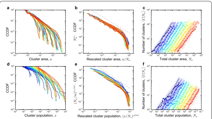
Extraction of urban clusters In the GRUMP data the spatial distribution of population is represented as a matrix, whose elements denote the estimated number of individuals resident within each of the grid cells. We apply a city clustering algorithm [10] (CCA) to the GRUMP data and define cities as spatial clusters of neighbouring grid cells with population over a given threshold,m, which also corresponds to the minimum cluster population. We vary the parametermover the interval [10–600] persons per km2, clustering adjacent cells with population above the thresholdm. As a reference, the official definition of urban area adopted by the United States census considers values ofmbetween 193 and 386 people per square kilometer [31]. In the range ofmconsidered, the numbers and sizes of clusters obtained with the CCA are very different. Panels b-d of Fig.4show the clusters within a square region in the Midwestern United States (Fig.4(a)) form= 28, 129, and 599. Both the number and areas of clusters decrease asmincreases and some large clusters split into multiple smaller clusters.
Global distribution of areas and populations of urban clusters Additionally, the gridded population data allows us to consider the area of urban clusters [32–34],a, as the rele-vant size variable, alternatively to population,x. Indeed, the distribution of urban areas is also known to follow Zipf ’s law with exponent α1, hence our null model predicts that the number of clusters is given by Equation (1), whereNnow denotes the total ur-banised area andαthe exponent of the distribution of city areas. The area and population of urban clusters are strongly correlated variables. The expansion of urban areas can be characterised by measuring the scaling relationship between the area,a, and population,
x, of the clusters. We use the gridded population data to measure urban sprawl for dif-ferent definitions of city, i.e. different values of the CCA parameterm(see Fig.4(e)). We observe that the scaling relationship betweenaandxhas the following dependence on the minimum population parameterm:
Figure 4Scaling properties of urban clusters. (a), Portion of the GRUMP dataset representing the distribution of population in a region of the Midwestern United States. The color denotes the logarithm of the population: light yellow for high population, dark blue for low population. (b)–(d), Urban clusters in the region depicted in panel (a) obtained applying the City Clustering Algorithm for different values of the minimum population parameter:m= 28 in (b), 129 in (c), 599 in (d). (e), Scaling relationship between area and population of clusters. The different colors denote different values of the CCA parameterm(see the legend of panel (f) for themvalues). The points indicate the average area of clusters with a given rescaled population. Data are fit to the power law in Equation (3) and the legend reports the values of the scaling exponentωfor the variousm. (f), Counter Cumulative Distribution Functions of cluster areas. The different colors denote different values of the CCA parameterm(see the legend for themvalues). The grey line is a power law with exponent –1 as a guide for the eye. (g), Counter Cumulative Distribution Functions of cluster populations,x(dashed curves), and rescaled populations, (x/m)ω(m)(solid curves). The grey line is a power law with exponent –1 as a guide for the eye
Note that the area of a cluster scales with the ratiox/m, which represents the maximum area that a cluster of populationxcan have, givenm. The scaling exponentωdepends onm. In particular,ω(m) is an increasing function ofm, which grows from 0.66 to 0.88. The sublinear scaling (ω(m) < 1 for allm) between a cluster’s area and population implies an increase in the population density of large clusters: the population density scales as
x/a=x1–ω, which is a growing function ofxwhen ω< 1. This result may support the
hypothesis on the economies of scale in the use of urban space. In fact, in large clusters space is organised more efficiently than in small clusters, so that each square kilometre of land can host a larger number of individuals, hence increasing the cluster’s population density [24]. Urban sprawl happens when the exponentωhas a large value, indicating a reduced efficiency in the utilisation of space as the size of clusters grows. The fact thatω
increases withmmeans that the estimated urban sprawl is bigger when clusters are defined using a largemand smaller whenmis small. The scaling relationship between area and population of clusters, Equation (3), implies that the Zipf exponents of the distributions of cluster areas and populations,αaandαxrespectively, are not independent, but related
by the equationαx=αa·ω(m).
The empirical distributions of cluster areas for different values of the CCA parameterm, shown in Fig.4(f ), indicate that the Zipf exponent for the areas isαa1, independent ofm.
The distributions of cluster populations, instead, have exponents that depend onm. If the populations are rescaled bymand elevated to the power ofω(m), the curves for different
Figure 5Zipf’s law and Heaps’ law for urban clusters. (a), Counter Cumulative Distribution Functions of areas of the clusters in all United States regions of 128×128 km2having urbanised area up to 5%. Regions are grouped in six groups according to their total urbanised area,Na, and the CCDFs of each group are computed separately for the different values of the CCA parameterm(see the legend in Fig.4(f ) for themvalues). (b), The CCDFs of panel (a) collapse on the same curve when the axes are properly rescaled. The dashed grey line is a power law with exponent –1 as a guide for the eye. (c), Average number of clusters as a function of the total urbanised area,Na, for the 128×128 km2United States regions (circles). The lower and upper values of the dashed areas denote the 10th and 90th percentile of 100 realisations of the null model. For clarity, curves have been shifted bym2along thex-axis. (d), Counter Cumulative Distribution Functions of populations of the clusters in all United States regions of 128×128 km2having urbanised area up to 5%. Regions are grouped in six groups according to their total population,Nx, and the CCDFs of each group are computed separately for the different values of the CCA parameterm. (e), The CCDFs of panel (d) collapse on the same curve when the axes are properly rescaled. The dashed grey line is a power law with exponent –1 as a guide for the eye. (f), Average number of clusters as a function of the total population,Nx, for the 128×128 km2 United States regions (circles). The lower and upper values of the dashed areas denote the 10th and 90th percentile of 100 realisations of the null model. For clarity, curves have been shifted bym2along thex-axis
Local distributions of areas and populations of urban clusters To understand how the number, areas and populations of clusters depend on the CCA parameterm, we perform a systematic analysis of the GRUMP data, considering regions at a smaller spatial scale. Our first result is that the assumptions of the null model hold locally for small regions of size 128×128 km2: the local distributions of city sizes are power laws with the same exponent as the global distribution at the country scale, with cutoffs that account for the finite sizes of the regions.
We divide the United States into non-overlapping square regions of sizeL= 128 km and obtain the urban clusters in each region applying the CCA for all values ofmbetween 10 and 600. We group together regions with similar total population,Nx, and built-up area,
Na, and compute the distributions of cluster sizes (i.e. populations and areas) separately
for each each group (see Fig.5(a), (d)). In order to avoid finite-size effects, we only con-sider regions with low urbanisation, having a percentage of built-up area smaller than 5% (this condition is satisfied by 49% of the regions form= 10 and up to 93% form= 599). If the assumptions of our null model hold, the Counter Cumulative Density Functions (CCDFs) of cluster areas and populations should be truncated power laws and have the formsP(>a|Na)∼a–αafa(a/Na) andP(>x|Nx)∼(x/m)–αx(m)fx(x/Nx), wherefa andfxare
for finite-size effects. The scaling collapses shown in Fig.5(b), (e) provide a validation to the predicted functional forms of the CCDFs.
Heap’s law for urban clusters Our second result is that the average number of clusters is related to the total size of the region as predicted by the null model and Equation (1). This means that cities are randomly distributed among the regions, even at small spatial scales. For each group of regions with similar total population,Nx, and built-up area,Na, we
compute the average number of clusters for all values of the CCA parameterm,C|Na,m
andC|Nx,m, and we check if these empirical values are compatible with the estimates
of the null model. To this end, we draw (with replacement) city areas and populations from the respective empirical distributions, until given target total values,NaandNx, are
reached. We repeat this procedure 100 times for increasing values ofNaandNx. For each
value of total area and population,NaandNx, we compute the mean number of cities
ob-tained for those total values,C|NaandC|Nx, and the confidence intervals defined as
the 10th and 90th percentiles of the number of clusters obtained in the 100 realisations. We observe that the empirical estimates of the average number of clusters lie within the null model’s confidence intervals (see Fig.5(c), (f )), confirming that empirical data is com-patible with a random distribution of clusters within the regions.
5 Conclusion
We empirically verified that a null model of urbanisation where cities are randomly dis-tributed in space produces correct estimates of the expected number of cities in regions of various sizes worldwide. This fact does not mean that cities are non-interacting and independent of each other. On the contrary, it is apparent that urban systems are strongly interacting [35]: internal migrations, for example, create a dependency in the dynamics of the population in various cities, with some cities increasing in size because others are decreasing. However, our analysis demonstrates that such interactions do not produce urbanisation patterns characterised by significant spatial correlations. It is important to highlight that this result has been obtained for regions of 128×128 km2in the United States, and further analysis on global urbanisation patterns at higher spatial resolution is needed to test the validity of this conclusion in other countries and at smaller spatial scales. Moreover, this result is expected to hold in regions where urbanisation is not too high. In the analysis of gridded population data we only consider regions with low ur-banisation, having a percentage of built-up area smaller than 5%. This is done because in highly urbanised areas deviations from Zipf ’s law and Heaps’ law are inevitable. In fact, in regions with large population density, urban clusters start to merge and, as a result, when population keeps increasing the number of clusters decreases instead of increases. Also, the distribution of cluster sizes loses its characteristic power law tail because of the emer-gence of one giant cluster. The characterisation of urban patterns in the regime of large population density requires the development of a different theoretical framework, which is a task left for future work.
The theoretical result relating the average number of cities to the total population, Equa-tion (1), is completely general and applicable to all systems characterised by Zipf ’s law for the distribution of group sizes, including word counts, the size of biological genera, the number of employees in firms and views/popularity of Youtube videos. Equation (1) is particularly useful in the analysis of finite-size systems in order to account for deviations from Heaps’ law.
Recently, Zipf ’s law has been shown to be connected to Taylor’s law, which describes the scaling between fluctuations in the size of a population and its mean [36]. This suggests the presence of a general connection between the three laws, Zipf ’s, Taylor’s and Heaps’ laws. Further research is needed to determine how the three laws can emerge from processes for the evolution of city sizes that incorporate birth, death and migration events.
Additional material
Additional file 1:Supplementary information (PDF 1.8 MB)
Acknowledgements
We thank J Grilli for insightful discussions.
Funding
FS is supported by EPSRC grant EP/P012906/1.
Abbreviations
GRUMP, Global Rural-Urban Mapping Project.
Availability of data and materials
TheGeonamesdataset analysed during the current study is available in the The GeoNames geographical database repository,http://download.geonames.org/export/dump/. TheGRUMPdataset analysed during the current study is available in the Socioeconomic Data and Applications Center (SEDAC) repository,
http://sedac.ciesin.columbia.edu/data/set/grump-v1-population-count.
Competing interests
The authors declare that they have no competing interests.
Authors’ contributions
FS and CJ analysed data and wrote the paper. All authors read and approved the final manuscript.
Publisher’s Note
Springer Nature remains neutral with regard to jurisdictional claims in published maps and institutional affiliations.
Received: 17 November 2017 Accepted: 27 June 2019
References
1. United Nations (1997) Principles and recommendations for population and housing censuses
2. Seto KC, Güneralp B, Hutyra LR (2012) Global forecasts of urban expansion to 2030 and direct impacts on biodiversity and carbon pools. Proc Natl Acad Sci 109(40):16083–16088
3. McNicoll G (2005) United Nations, Department of Economic and Social Affairs: world economic and social survey 2004: international migration. Popul Dev Rev 31(1):183–185
4. Angel S, Parent J, Civco DL, Blei A, Potere D (2011) The dimensions of global urban expansion: estimates and projections for all countries, 2000–2050. Prog Plann 75(2):53–107
5. Auerbach F (1913) Das gesetz der bevölkerungskonzentration. Petermanns Geogr Mitt 59:74–76 6. Zipf GK (1935) The psycho-biology of language. Houghton, Mifflin, Oxford
7. Ioannides YM, Overman HG (2003) Zipf’s law for cities: an empirical examination. Reg Sci Urban Econ 33(2):127–137 8. Rybski D, Ros AGC, Kropp JP (2013) Distance-weighted city growth. Phys Rev E 87(4):042114
9. Makse HA, Havlin S, Stanley H (1995) Modelling urban growth. Nature 377(1912):779–782
10. Rozenfeld HD, Rybski D, Andrade JS, Batty M, Stanley HE, Makse HA (2008) Laws of population growth. Proc Natl Acad Sci 105(48):18702–18707
11. Frasco GF, Sun J, Rozenfeld HD, Ben-Avraham D (2014) Spatially distributed social complex networks. Phys Rev X 4(1):011008
13. Leyvraz F, Redner S (2002) Scaling theory for migration-driven aggregate growth. Phys Rev Lett 88(6):068301 14. Marsili M, Zhang YC (1998) Interacting individuals leading to Zipf’s law. Phys Rev Lett 80(12):2741
15. Gabaix X (1999) Zipf’s law for cities: an explanation. Q J Econ 114(3):739–767 16. Eeckhout J (2004) Gibrat’s law for (all) cities. Am Econ Rev 94(5):1429–1451
17. Gabaix X, Ioannides YM (2004) The evolution of city size distributions. In: Handbook of regional and urban economics, vol 4, pp 2341–2378
18. Gibrat R (1931) Les inégalités économiques. Recueil Sirey, France
19. Hernando A, Hernando R, Plastino A, Zambrano E (2015) Memory-endowed US cities and their demographic interactions. J R Soc Interface 12(102):20141185
20. Heaps HS (1978) Information retrieval: computational and theoretical aspects. Academic Press, San Diego 21. Gerlach M, Altmann EG (2014) Scaling laws and fluctuations in the statistics of word frequencies. New J Phys
16(11):113010
22. Lü L, Zhang ZK, Zhou T (2010) Zipf’s law leads to Heaps’ law: analyzing their relation in finite-size systems. PLoS ONE 5(12):e14139
23. Azaele S, Suweis S, Grilli J, Volkov I, Banavar JR, Maritan A (2016) Statistical mechanics of ecological systems: neutral theory and beyond. Rev Mod Phys 88(3):035003
24. Bettencourt LM (2013) The origins of scaling in cities. Science 340(6139):1438–1441
25. Arcaute E, Hatna E, Ferguson P, Youn H, Johansson A, Batty M (2015) Constructing cities, deconstructing scaling laws. J R Soc Interface 12(102):20140745
26. Vatant B, Wick M (2012) Geonames ontology
27. The World Bank, World Development Indicators (2010) Available from:http://data.worldbank.org/data
28. Christaller W (1933) Die zentralen Orte in Süddeutschland: eine ökonomisch-geographische Untersuchung über die Gesetzmässigkeit der Verbreitung und Entwicklung der Siedlungen mit städtischen Funktionen. University Microfilms
29. Lösch A (1940) Die räumliche Ordnung der Wirtschaft: eine Untersuchung über Standort. Wirtschaftsgebiete und internationalen Handel, Verlag Wirtschaft und Finanzen. Jena
30. Center for International Earth Science Information Network CUFPRIWBCIdAT (2007) Global rural urban mapping project (GRUMP) alpha: gridded population of the world, version 2, with urban reallocation (GPW-UR)
31. Ratcliffe M, Burd C, Holder K, Fields A (2016) Defining rural at the US Census Bureau. American Community Survey and Geography Brief
32. Batty M, Longley PA (1994) Fractal cities: a geometry of form and function. Academic Press, San Diego 33. Lemoy R, Caruso G (2018) Evidence for the homothetic scaling of urban forms. In: Environment and planning B:
urban analytics and city science p 2399808318810532
34. Nordbeck S (1971) Urban allometric growth. Geogr Ann, Ser B, Hum Geogr 53(1):54–67
35. Hernando A, Hernando R, Plastino A (2013) Space-time correlations in urban sprawl. J R Soc Interface 11(91):20130930