Structure from motion using dense CNN features with keypoint relocalization

E X P R E S S P A P E R

Open Access

Structure from motion using dense CNN

features with keypoint relocalization

Aji Resindra Widya

, Akihiko Torii and Masatoshi Okutomi

Abstract

Structure from motion (SfM) using imagery that involves extreme appearance changes is yet a challenging task due to a loss of feature repeatability. Using feature correspondences obtained by matching densely extracted convolutional neural network (CNN) features significantly improves the SfM reconstruction capability. However, the reconstruction accuracy is limited by the spatial resolution of the extracted CNN features which is not even pixel-level accuracy in the existing approach. Providing dense feature matches with precise keypoint positions is not trivial because of memory limitation and computational burden of dense features. To achieve accurate SfM reconstruction with highly

repeatable dense features, we propose an SfM pipeline that uses dense CNN features with relocalization of keypoint position that can efficiently and accurately provide pixel-level feature correspondences. Then, we demonstrate on the Aachen Day-Night dataset that the proposed SfM using dense CNN features with the keypoint relocalization

outperforms a state-of-the-art SfM (COLMAP using RootSIFT) by a large margin.

Keywords: Structure from Motion, Feature detection and description, Feature matching, 3D reconstruction

1 Introduction

Structure from motion (SfM) is getting ready for 3D reconstruction only using images, thanks to off-the-shelf softwares [1–3] and open-source libraries [4–10]. They provide impressive 3D models, especially, when targets are captured from many viewpoints with large over-laps. The state-of-the-art SfM pipelines, in general, start with extracting local features [11–17] and matching them across images, followed by pose estimation, triangulation, and bundle adjustment [18–20]. The performance of local features and their matching, therefore, is crucial for 3D reconstruction by SfM.

In this decade, the performance of local features, namely, SIFT [11] and its variants [16, 21–24] are vali-dated on 3D reconstruction as well as many other tasks [25–27]. The local features give promising matches for well-textured surfaces/objects but significantly drop its performance for matching weakly textured objects [28], repeated patterns [29], extreme changes of viewpoints [21, 30,31], and illumination change [32,33] because of degradation in repeatability of feature point (keypoint) extraction [21, 31]. This problem can be mitigated by

*Correspondence:[email protected]

Tokyo Institute of Technology, O-okayama, Meguro-ku, 152-8550 Tokyo, Japan

using densely detected features on a regular grid [34,35] but their merit is only demonstrated in image retrieval [32, 36] or image classification tasks [26, 34] that use the features for global image representation and do not require one-to-one feature correspondences as in SfM.

Only recently, SfM with densely detected features are presented in [37]. DenseSfM [37] uses convolutional neu-ral network (CNN) features as densely detected features, i.e., it extracts convolutional layers of deep neural network [38] and converts them as feature descriptors of keypoints on a grid pattern (Section3.1). As the main focus of [37] is camera localization, the SfM architecture including nei-ther dense CNN feature description and matching nor its 3D reconstruction performance is not studied in detail.

1.1 Contribution

In this work, we first review the details of the SfM pipeline with dense CNN feature extraction and matching. We then propose a keypoint relocalization that uses the struc-ture of convolutional layers (Section 3.2) to overcome keypoint inaccuracy on the grid resolution and compu-tational burden of dense feature matching. Finally, the performance of SfM with dense CNN feature using the proposed keypoint relocalization is evaluated on Aachen

Day-Night [37] dataset and additionally on Strecha [39] dataset.

2 Related work

2.1 SfM and VisualSLAM

The state-of-the-art SfM is divided into a few mainstream pipelines: incremental (or sequential) [4,6,40], global [8, 9,41], and hybrid [10,42].

VisualSLAM approaches, namely, LSD-SLAM [43] and DTAM [44], repeat camera pose estimation based on selected keyframe and (semi-)dense reconstruction using the pixel-level correspondences in real-time. These meth-ods are particularly designed to work with video streams, i.e., short baseline camera motion, but not with general wide-baseline camera motion.

Recently, Sattler et al. [37] introduces CNN-based Dens-eSfM that adopts densely detected and described features. But their SfM uses fixed poses and intrinsic parameters of reference images in evaluating the performance of query image localization. They also do not address keypoint inaccuracy of CNN features. Therefore, it remains as an open challenge.

2.2 Feature points

The de facto standard local feature, SIFT [11], is capa-ble of matching images under viewpoint and illumination changes thanks to scale and rotation invariant keypoint patches described by histograms of the oriented gradi-ent. ASIFT [21] and its variants [30,31] explicitly generate synthesized views in order to improve repeatability of key-point detection and description under extreme viewkey-point changes.

An alternative approach to improve feature matching between images across extreme appearance changes is to use densely sampled features from images. Densely detected features are often used in multi-view stereo [45] with DAISY [46], or image retrieval and classification [35, 47] with Dense SIFT [34]. However, dense features are not spotlighted in the task of one-to-one feature cor-respondence search under unknown camera poses due to

its loss of scale, rotation invariant, inaccuracy of localized keypoints, and computational burden.

2.3 CNN features

Fischer et al. [48] reported that, given feature positions, descriptors extracted from CNN layer have better match-ability compared to SIFT [11]. More recently, Schon-berger et al. [49] also showed that CNN-based learned local features such as LIFT [17],Deep-Desc[50], and Con-vOpt [51] have higher recall compared to SIFT [11] but still cannot outperform its variants, e.g., DSP-SIFT [16] and SIFT-PCA [52].

Those studies motivate us to adopt CNN architecture for extracting features from images and matching them for SfM as it efficiently outputs multi-resolution features and has potential to be improved by better training or architecture.

3 The pipeline: SfM using dense CNN features with keypoint relocalization

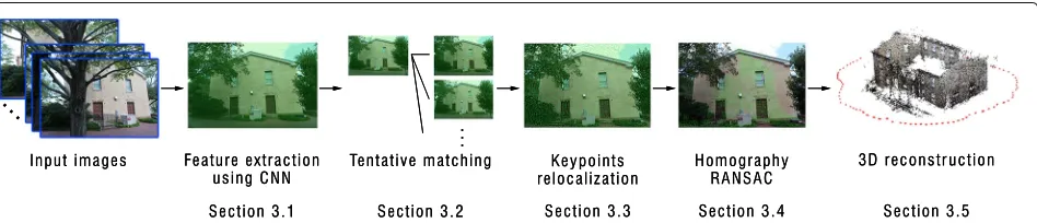
Our SfM using densely detected features mimics the state-of-the-art incremental SfM pipeline that con-sists of feature extraction (Section 3.1), feature match-ing (Section 3.2 to 3.4), and incremental reconstruc-tion (Secreconstruc-tion 3.5). Figure 1 overviews the pipeline. In this section, we describe each component while stating the difference to the sparse keypoint-based approaches.

3.1 Dense feature extraction

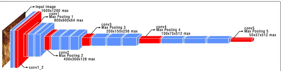
Firstly, our method densely extracts the feature descrip-tors and their locations from the input image. In the same spirit of [53,54], we input images in a modern CNN archi-tecture [38, 55, 56] and use the convolutional layers as densely detected keypoints on a regular grid, i.e., crop-ping out the fully connected and softmax layers. In the following, we chose VGG-16 [38] as the base network architecture and focus on the description tailored to it, but this can be replaced with other networks with marginal modification.

As illustrated in Fig.2, VGG-16 [38] is composed of five max-pooling layers and 16 weight layers. We extract the max-pooling layers as dense features. As can be seen in Fig. 2, the conv1 max-pooling layer is not yet the same resolution as the input image. We, therefore, also extract conv1_2, one layer before the conv1 max-pooling layer, that has pixel-level accuracy.

3.2 Tentative matching

Given multi-level feature point locations and descriptors, tentative matching uses upper max-pooling layer (lower spatial resolution) to establish initial correspondences. This is motivated by that the upper max-pooling layer has a larger receptive field and encodes more seman-tic information [48,57, 58] which potentially gives high matchability across appearance changes. Having the lower spatial resolution is also advantageous in the sense of computational efficiency.

For a pair of images, CNN descriptors are tentatively matched by searching their nearest neighbors (L2 dis-tances) and refined by taking mutually nearest neighbors. Note that the standard ratio test [11] removes too many feature matches as neighborhood features on a regularly sampled grid tend to be similar to each other.

We perform feature descriptor matching for all the pairs of images or shortlisted images by image retrieval, e.g., NetVLAD [53].

3.3 Keypoint relocalization

The tentative matching using the upper max-pooling lay-ers, e.g., conv5, generates distinctive correspondences but the accuracy of keypoint position is limited by their spatial resolution. This inaccuracy of keypoints can be mitigated by a coarse-to-fine matching from the extracted max-pooling layer up to conv1_2 layer utilizing extracted inter-mediate max-pooling layers between them. For exam-ple, the matched keypoints found on the conv3 layer are transferred to the conv2 (higher spatial resolution) and new correspondences are searched only in the area

constrained by the transferred keypoints. This can be repeated until reaching conv1_2 layer. However, this naive coarse-to-fine matching generates too many keypoints that may lead to a problem in computational and mem-ory usage in incremental SfM step, especially, bundle adjustment.

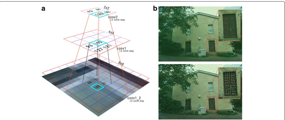
To generate dense feature matches with pixel-level accu-racy while preserving their quantity, we propose a method of keypoint relocalization as follows. For each feature point at the current layer, we retrieve the descriptors on the lower layer (higher spatial resolution) in the corre-spondingK×Kpixels1. The feature point is relocalized at the pixel position that has the largest descriptor norm (L2 norm) in theK×Kpixels. This relocalization is repeated until it reaches the conv1_2 layer which has the same resolution as the input image (see also Fig.3).

3.4 Feature verification using RANSAC with multiple homographies

Using all the relocated feature points, we next remove outliers from a set of tentative matches by Homography-RANSAC. We rather use a vanilla RANSAC instead of the state-of-the-art spatial verification [59] by taking into account the spatial density of feature correspon-dences. To detect inlier matches lying on several planes, Homography-RANSAC is repeated while excluding the inlier matches of the best hypothesis. The RANSAC inlier/outlier threshold is set to be loose to allow features off the planes.

3.5 3D reconstruction

Having all the relocalized keypoints filtered by RANSAC, we can export them to any available pipelines that per-form pose estimation, point triangulation, and bundle adjustment.

Dense matching may produce many confusing feature matches on the scene with many repetitive structures, e.g., windows, doors, and pillars. In such cases, we keep only the N best matching image pairs for each image in the

Fig. 3Keypoint relocalization.aA keypoint on a sparser level is relocalized using a map computed from descriptors’ L2 norm on an lower level which has higher spatial resolution. It is reassigned at the position on the lower level which has the largest value in the correspondingK_×K

neighborhood. By repeating this, the relocalized keypoint position in conv1_2 has the accuracy as in the input image pixels.bThe green dots show the extracted conv3 features points (top) and the result of our keypoint relocalization (bottom)

dataset based on the number of inlier matches of multiple Homography-RANSAC.

4 Experiments

We implement feature detection, description, and match-ing (Sections 3.1 to 3.4) in MATLAB with third-party libraries (MatConvNet [60] and Yael library [61]). Dense CNN features are extracted using the VGG-16 network [38]. Using conv4 and conv3 max-pooling layers, feature matches are computed by the coarse-to-fine matching fol-lowed by multiple Homography-RANSAC that finds at most five homographies supported by an inlier thresh-old of 10 pixels. The best N pairs based on multiple Homography-RANSAC of every image are imported to COLMAP [6] with the fixed intrinsic parameter option for scene with many repetitive structures. Otherwise, we use all the image pairs.

In our preliminary experiments, we tested other lay-ers having the same spatial resolution, e.g., using conv4_3 and conv3_3 layers in the coarse-to-fine matching but we observed no improvement in 3D reconstruction. As a max-pooling layer has a half depth dimension in compar-ison with the other layers at the same spatial resolution, we chose the max-pooling layer as the dense features for efficiency.

In the following, we evaluate the reconstruction per-formance on Aachen Day-Night [37] and Strecha [39] dataset. We compare our SfM using dense CNN features with keypoint relocalization to the baseline COLMAP with DoG+RootSIFT features [6]. In addition, we also compare our SfM to SfM using dense CNN without keypoint relocalization [37]. All experiments are tested

on a computer equipped with a 3.20-GHz Intel Core i7-6900K CPU with 16 threads and a 12-GB GeForce GTX 1080Ti.

4.1 Results on Aachen Day-Night dataset

The Aachen Day-Night dataset [37] is aimed for evaluat-ing SfM and visual localization under large illumination changes such as day and night. It includes 98 subsets of images. Each subset consists of 20 day-time images and one night-time image, their reference camera poses, and 3D points2.

For each subset, we run SfM and evaluate the esti-mated camera pose of the night image as follows. First, the reconstructed SfM model is registered to the ref-erence camera poses by adopting a similarity transform obtained from the camera positions of day-time images. We then evaluate the estimated camera pose of the night image by measuring positional (L2 distance) and angular

(acos(trace(RrefR

T night)−1 2 )) error.

Table 1 shows the number of reconstructed cameras. The proposed SfM with keypoint relocalization (conv1_2)

Table 1Number of cameras reconstructed on the Aachen dataset

DoG+ DenseCNN DenseCNN

RootSIFT [6] w/o reloc w/ reloc (Ours)

Night 48 95 96

Day 1910 1924 1944

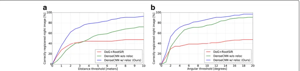
Fig. 4Quantitative evaluation on the Aachen Day-Night dataset. The poses of night images reconstructed by the baseline DoG+RootSIFT [6] (red), the DenseCNN without keypoint relocalization (green), and the proposed DenseCNN (blue) are evaluated using the reference poses. The graphs show the percentages of correctly reconstructed camera poses of night images (y-axis) at positional (a) and angular (b) error threshold (x-axis)

can reconstruct 96 night images that are twice as many as that of the baseline method using COLMAP with DoG+RootSIFT [6]. This result validates the benefit of densely detected features that can provide correspon-dences across large illumination changes as they have smaller loss in keypoint detection repeatability than a standard DoG. On the other hand, both methods with sparse and dense features work well for reconstructing day images. The difference between with and without key-point localization can be seen more clearly in the next evaluation.

Figure4shows the percentages of night images recon-structed (y-axis) within certain positional and angular error threshold (x-axis). Similarly, Table 2 shows the reconstruction percentages of night images for vary-ing distance error thresholds with a fixed angular error threshold at 10°. As can be seen from both evaluations, the proposed SfM using dense CNN features with keypoint relocalization outperforms the baseline DoG+RootSIFT [6] by a large margin. The improvement by the proposed keypoint relocalization is significant when the evalua-tion accounts for pose accuracy. Notice that the SfM using dense CNN without keypoint relocalization [37] performs worse than the baseline DoG+RootSIFT [6] at small thresholds, e.g., below 3.5 m position and 2◦angular error. This indicates that the proposed keypoint relocal-ization gives features at more stable and accurate posi-tions and provides better inlier matches for COLMAP reconstruction which results 3D reconstruction in higher quality.

Figure 5 illustrates the qualitative comparison result between our method and the baseline DoG+RootSIFT [6].

4.2 Results on Strecha dataset

We additionally evaluate our SfM using dense CNN with the proposed keypoint relocalization on all six subsets of Strecha dataset [39] which is a standard benchmark dataset for SfM and MVS. Position and angular error between the reconstructed cameras and the ground truth

poses are evaluated. In our SfM, we take only feature matches from the bestN = 5 image pairs for each image to suppress artifacts from confusing image pairs.

The mean average position and angular errors resulted by our SfM are 0.59 m and 2.27◦. Although these errors are worse than those of the state-of-the-art COLMAP with DoG+RootSIFT [6] which are 0.17 m and 0.90◦, the quantitative evaluation on the Strecha dataset demon-strated that our SfM does not overfit to specific challeng-ing tasks but works reasonably well for standard (easy) situations.

5 Conclusion

We presented a new SfM using dense features extracted from CNN with the proposed keypoint relocalization to improve the accuracy of feature positions sampled on a regular grid. The advantage of our SfM has demonstrated on the Aachen Day-Night dataset that includes images with large illumination changes. The result on the Strecha dataset also showed that our SfM works for standard datasets and does not overfit to a particular task although it is less accurate than the state-of-the-art SfM with local features. We wish the proposed SfM becomes a mile-stone in the 3D reconstruction, in particularly challenging situations.

Table 2Evaluation of reconstructed camera poses (both position and orientation)

DoG+ DenseCNN DenseCNN

RootSIFT [6] w/o reloc w/ reloc (Ours)

0.5m 15.31 5.10 18.37

1.0m 25.61 14.29 33.67

5.0m 36.73 45.92 69.39

10.0m 35.71 61.22 81.63

20.0m 39.80 69.39 82.65

The numbers show the percentage of the reconstructed night images within given positional error thresholds and an angular error fixed at 10°

Fig. 5Example of 3D reconstruction in the Aachen dataset. These figures show qualitative examples of SfM using DoG+RootSIFT [6] (a) and our dense CNN with keypoint relocalization (b). Our method can reconstruct all the 21 images in the subset whereas the baseline DoG+RootSIFT [6] fails to reconstruct it. As a nature of dense feature matching, our method reconstructs 42,402 3D points which are 8.2 times more than the baseline method

Endnotes

1_{We useK =2 throughout the experiments.}

2_{Although the poses are carefully obtained with manual}

verification, the poses are called as “reference poses” but not ground truth.

Acknowledgements

This work was partly supported by JSPS KAKENHI Grant Number 17H00744, 15H05313, 16KK0002, and Indonesia Endowment Fund for Education.

Availability of data and materials

The code will be made publicly available on acceptance.

Authors’ contributions

AR run all the experiment and wrote initial draft of the manuscript. AT revised the manuscript. Both AT and MXO provided supervision, many meaningful discussion, and guidance to AR in this research. All authors read and approved the final manuscript.

Competing interests

The authors declare that they have no competing interests.

Publisher’s Note

Springer Nature remains neutral with regard to jurisdictional claims in published maps and institutional affiliations.

Received: 14 March 2018 Accepted: 6 May 2018

References

1. Pix4D - Professional drone mapping and photogrammetry software.

https://pix4d.com/. Accessed 11 Feb 2018

2. Agisoft Photoscan.http://www.agisoft.com/. Accessed 11 Feb 2018 3. Discover Photogrammetry Software - Photomodeler.http://www.

photomodeler.com/index.html. Accessed 11 Feb 2018 4. Fuhrmann S, Langguth F, Goesele M (2014) MVE-A Multi-View

Reconstruction Environment. In: GCH. Eurographics Association, Aire-la-Ville. pp 11–18

5. Sweeney C, Hollerer T, Turk M (2015) Theia: A fast and scalable structure-from-motion library. In: Proc. ACMM. ACM, New York. pp 693–696

6. Schonberger JL, Frahm JM (2016) Structure-from-motion revisited. In: Proc. CVPR. IEEE. pp 4104–4113

7. Schönberger JL, Zheng E, Frahm JM, Pollefeys M (2016) Pixelwise view selection for unstructured multi-view stereo. In: Proc. ECCV. Springer, Cham. pp 501–518

8. Wilson K, Snavely N (2014) Robust global translations with 1dsfm. In: Proc. ECCV. Springer, Cham. pp 61–75

9. Moulon P, Monasse P, Perrot R, Marlet R (2016) OpenMVG: Open multiple view geometry. In: International Workshop on Reproducible Research in Pattern Recognition. Springer, Cham. pp 60–74

10. Cui H, Gao X, Shen S, Hu Z (2017) Hsfm: Hybrid structure-from-motion. In: Proc. CVPR. IEEE, Boston. pp 2393-2402

11. Lowe DG (2004) Distinctive image features from scale-invariant keypoints. IJCV 60(2):91–110

12. Mikolajczyk K, Schmid C (2004) Scale & affine invariant interest point detectors. IJCV 60(1):63–86

13. Kadir T, Zisserman A, Brady M (2004) An affine invariant salient region detector. In: Proc. ECCV. Springer, Cham. pp 228–241

14. Tuytelaars T, Van Gool L (2004) Matching widely separated views based on affine invariant regions. IJCV 59(1):61–85

15. Arandjelovi´c R, Zisserman A (2012) Three things everyone should know to improve object retrieval. In: Proc. CVPR. IEEE, Providence. pp 2911–2918 16. Dong J, Soatto S (2015) Domain-size pooling in local descriptors: Dsp-sift.

In: Proc. CVPR. IEEE, Boston. pp 5097–5106

17. Yi KM, Trulls E, Lepetit V, Fua P (2016) Lift: Learned invariant feature transform. In: Proc. ECCV. Springer, Cham. pp 467–483

18. Snavely N, Seitz SM, Szeliski R (2008) Modeling the world from internet photo collections. IJCV 80(2):189–210

19. Agarwal S, Furukawa Y, Snavely N, Curless B, Seitz SM, Szeliski R (2010) Reconstructing rome. Computer 43(6):40–47

20. Agarwal S, Furukawa Y, Snavely N, Simon I, Curless B, Seitz SM, Szeliski R (2011) Building rome in a day. Commun ACM 54(10):105–112 21. Morel JM, Yu G (2009) Asift: A new framework for fully affine invariant

image comparison. SIAM J Imaging Sci 2(2):438–469

22. Ke Y, Sukthankar R (2004) Pca-sift: A more distinctive representation for local image descriptors. In: Proc. CVPR, vol 2. IEEE, Washington

23. Abdel-Hakim AE, Farag AA (2006) Csift: A sift descriptor with color invariant characteristics. In: Proc. CVPR, vol, 2. IEEE, New York. pp 1978–1983 24. Bay H, Tuytelaars T, Van Gool L (2006) Surf: Speeded up robust features. In:

Proc. ECCV. Springer, Cham. pp 404–417

25. Csurka G, Dance C, Fan L, Willamowski J, Bray C (2004) Visual categorization with bags of keypoints. In: Proc. ECCV, vol 1. Springer, Cham. pp 1–2

26. Lazebnik S, Schmid C, Ponce J (2006) Beyond bags of features: Spatial pyramid matching for recognizing natural scene categories. In: Proc. CVPR, vol 2. IEEE, New York. pp 2169–2178

27. Chong W, Blei D, Li FF (2009) Simultaneous image classification and annotation. In: Computer Vision and Pattern Recognition, 2009. CVPR 2009. IEEE Conference On. IEEE, Miami. pp 1903–1910

28. Hinterstoisser S, Cagniart C, Ilic S, Sturm P, Navab N, Fua P, Lepetit V (2012) Gradient response maps for real-time detection of textureless objects. IEEE PAMI 34(5):876–888

29. Torii A, Sivic J, Pajdla T, Okutomi M (2013) Visual place recognition with repetitive structures. In: Proc. CVPR. IEEE, Portland. pp 883–890 30. Mishkin D, Matas J, Perdoch M (2015) Mods: Fast and robust method for

31. Taira H, Torii A, Okutomi M (2016) Robust feature matching by learning descriptor covariance with viewpoint synthesis. In: Proc. ICPR. IEEE, Cancun. pp 1953–1958

32. Torii A, Arandjelovi´c R, Sivic J, Okutomi M, Pajdla T (2015) 24/7 place recognition by view synthesis. In: Proc. CVPR. IEEE, Boston. pp 1808–1817 33. Radenovic F, Schonberger JL, Ji D, Frahm JM, Chum O, Matas J (2016)

From dusk till dawn: Modeling in the dark. In: Proc. CVPR. IEEE, Las Vegas. pp 5488–5496

34. Bosch A, Zisserman A, Munoz X (2007) Image classification using random forests and ferns. In: Proc. ICCV. IEEE, Rio de Janeiro. pp 1–8

35. Liu C, Yuen J, Torralba A (2016) Sift flow: Dense correspondence across scenes and its applications. In: Dense Image Correspondences for Computer Vision. Springer, Cham. pp 15–49

36. Zhao WL, Jégou H, Gravier G (2013) Oriented pooling for dense and non-dense rotation-invariant features. In: Proc. BMVC. BMVA, South Road 37. Sattler T, Maddern W, Toft C, Torii A, Hammarstrand L, Stenborg E, Safari D,

Sivic J, Pajdla T, Pollefeys M, Kahl F, Okutomi M (2017) Benchmarking 6dof outdoor visual localization in changing conditions. arXiv preprint arXiv:1707.09092

38. Simonyan K, Zisserman A (2014) Very deep convolutional networks for large-scale image recognition. arXiv preprint arXiv:1409.1556 39. Strecha C, Von Hansen W, Van Gool L, Fua P, Thoennessen U (2008) On

benchmarking camera calibration and multi-view stereo for high resolution imagery. In: Proc. CVPR. IEEE, Anchorage. pp 1–8

40. Wu C (2013) Towards linear-time incremental structure from motion. In: Proc. 3DV. IEEE, Seattle. pp 127–134

41. Cui Z, Tan P (2015) Global structure-from-motion by similarity averaging. In: Proc. ICCV. IEEE, Santiago. pp 864–872

42. Magerand L, Del Bue A (2017) Practical projective structure from motion (p2sfm). In: Proc. CVPR. IEEE, Venice. pp 39–47

43. Engel J, Schöps T, Cremers D (2014) Lsd-slam: Large-scale direct monocular slam. In: Proc. ECCV. Springer, Cham. pp 834–849 44. Newcombe RA, Lovegrove SJ, Davison AJ (2011) Dtam: Dense tracking

and mapping in real-time. In: Proc. ICCV. IEEE, Barcelona. pp 2320–2327 45. Furukawa Y, Hernández C, et al (2015) Multi-view stereo: A tutorial. Found

Trends® Comput Graph Vis 9(1-2):1–148

46. Tola E, Lepetit V, Fua P (2010) Daisy: An efficient dense descriptor applied to wide-baseline stereo. IEEE PAMI 32(5):815–830

47. Tuytelaars T (2010) Dense interest points. In: Proc. CVPR. IEEE, San Francisco. pp 2281–2288

48. Fischer P, Dosovitskiy A, Brox T (2014) Descriptor matching with convolutional neural networks: a comparison to sift. arXiv preprint arXiv:1405.5769

49. Schonberger JL, Hardmeier H, Sattler T, Pollefeys M (2017) Comparative evaluation of hand-crafted and learned local features. In: Proc. CVPR. IEEE, Honolulu. pp 6959–6968

50. Simo-Serra E, Trulls E, Ferraz L, Kokkinos I, Fua P, Moreno-Noguer F (2015) Discriminative learning of deep convolutional feature point descriptors. In: Proc. ICCV. IEEE, Santiago. pp 118–126

51. Simonyan K, Vedaldi A, Zisserman A (2014) Learning local feature descriptors using convex optimisation. IEEE PAMI 36(8):1573–1585 52. Bursuc A, Tolias G, Jégou H (2015) Kernel local descriptors with implicit

rotation matching. In: Proc. ACMM. ACM, New York. pp 595–598 53. Arandjelovic R, Gronat P, Torii A, Pajdla T, Sivic J (2016) NetVLAD: CNN

architecture for weakly supervised place recognition. In: Proc. CVPR. IEEE, Las Vegas. pp 5297–5307

54. Radenovi´c F, Tolias G, Chum O (2016) CNN image retrieval learns from BoW: Unsupervised fine-tuning with hard examples. In: Proc. ECCV. Springer, Cham

55. Szegedy C, Liu W, Jia Y, Sermanet P, Reed S, Anguelov D, Erhan D, Vanhoucke V, Rabinovich A, et al. (2015) Going deeper with convolutions. In: Proc. CVPR, Boston

56. He K, Zhang X, Ren S, Sun J (2016) Deep residual learning for image recognition. In: Proc. CVPR. IEEE, Las Vegas. pp 770–778

57. Berkes P, Wiskott L (2006) On the analysis and interpretation of inhomogeneous quadratic forms as receptive fields. Neural Comput 18(8):1868–1895

58. Zeiler MD, Fergus R (2014) Visualizing and understanding convolutional networks. In: European Conference on Computer Vision. Springer, Cham. pp 818–833

59. Philbin J, Chum O, Isard M, Sivic J, Zisserman A (2007) Object retrieval with large vocabularies and fast spatial matching. In: Proc. CVPR. IEEE, Minneapolis

60. Vedaldi A, Lenc K (2015) Matconvnet – convolutional neural networks for matlab. In: Proc. ACMM. ACM, New York

61. Douze M, Jégou H (2014) The yael library. In: Proc. ACMM. MM ’14. ACM, New York, USA. pp 687–690.https://doi.org/10.1145/2647868.2654892.