Resolving intravoxel white matter structures
in the human brain using regularized regression
and clustering
Andrea Hart
1, Brianna Smith
1, Sean Smith
1, Elijah Sales
1, Jacqueline Hernandez‑Camargo
1, Yarlin Mayor Garcia
1,
Felix Zhan
1, Lori Griswold
2, Brian Dunkelberger
2, Michael R. Schwob
3, Sharang Chaudhry
3, Justin Zhan
3*,
Laxmi Gewali
3and Paul Oh
3Introduction
The human brain is primarily composed of neural tissue, which is responsible for receiv-ing and relayreceiv-ing electrical impulses for a variety of purposes. Neuronal cells (neurons) have three primary components: a cell body which contains all of its organelles, the sig-nal input structures (dendrites), and the sigsig-nal output structures (axons). Typically, den-drites are much shorter projections than axons. Denden-drites and cell bodies are located on the outer edges of the brain and are collectively called grey matter. Axons, referred to as white matter, tend to be interior to grey matter [1].
The brain exhibits functional specialization, causing axons to traverse the brain from one functional group to another, relaying information. As this information fre-quently requires more than one axon to relay the complete signal, many axons are
grouped together in fiber tracts known as nerves [2]. Nerves within the body are
eas-ily distinguishable due to their length and separation from other neural tissue. How-ever, the sheer amount of neuropil that cross and intertwine within the white matter makes it extremely difficult to uniquely isolate and identify individual nerves and their paths within the brain. Adding to this complexity, neural pathfinding is not so highly correlated from one brain to the next; moreover, it would be difficult to get a
Abstract
The human brain is a complex system of neural tissue that varies significantly between individuals. Although the technology that delineates these neural pathways does not currently exist, medical imaging modalities, such as diffusion magnetic resonance imaging (dMRI), can be leveraged for mathematical identification. The purpose of this work is to develop a novel method employing machine learning techniques to determine intravoxel nerve number and direction from dMRI data. The method was tested on multiple synthetic datasets and showed promising estimation accuracy and robustness for multi‑nerve systems under a variety of conditions, including highly noisy data and imprecision in parameter assumptions.
Keywords: Ball‑and‑stick model, Diffusion MRI, Tractography, Nerve, Neural tracts, Brain imaging
Open Access
© The Author(s) 2019. This article is distributed under the terms of the Creative Commons Attribution 4.0 International License (http://creat iveco mmons .org/licen ses/by/4.0/), which permits unrestricted use, distribution, and reproduction in any medium, provided you give appropriate credit to the original author(s) and the source, provide a link to the Creative Commons license, and indicate if changes were made.
RESEARCH
clear picture of any one person’s brain by analyzing another’s [3]. Although the exact technology that delineates these neural pathways does not exist at this time, current medical imaging modalities, such as dMRI, can be leveraged for this purpose.
Diffusion magnetic resonance imaging (dMRI) relies on the temporary application of a magnetic field applied in several gradient directions to excite water molecules, causing molecular reorientation and motion, and ultimately creating detectable
sig-nals [4]. The reorientation of water molecules is restricted by the tissue composition;
therefore, a baseline signal is achieved based on how much water is localized within a subregion of the brain. In addition, the motion caused by the gradients in the mag-netic field dampens these baseline signals. This ultimately allows dMRI to provide insight into the microscopic details of tissue architecture and allows the mapping of white matter tracts throughout the brain. Furthermore, an impactful aspect of using dMRI for tracing neural pathways is that it can be done non-invasively and in-vivo using mathematical modeling. Applications of tracking white matter include treat-ment and managetreat-ment of traumatic brain injuries, neurodegenerative diseases, and pre-surgical visualization of the brain [5].
Data from dMRI are collected for small artificially-divided subregions in the brain called volumetric pixels, or voxels. Voxels are cubes of side length 1–3 mm and form a 3-dimensional grid for picturing the brain. This is similar to visualizing images in 2-dimensions with pixels. The overall problem of mapping neural pathways can be thought of, mathematically, as resolving white matter structures for all voxels within the brain. Using dMRI data for understanding intravoxel white matter structure is a mathematically challenging problem. Several strategies have been proposed in
lit-erature [6–21]. Additionally, the difficulty is increased given that there is no
“gold-standard” for evaluating the process.
Several novel methods exist to detect neural fiber orientation using dMRI data. Additionally, there have been multiple attempts to obtain high angular resolution of white matter fiber. Though the objectives of these methods seem related, there does not yet exist a method to combine these efforts and resolve intravoxel white matter structures in regards to both orientation and concentration.
The proposed method attempts to resolve white matter with robust accuracy using elastic net and clustering techniques. Compared to existing methods, the proposed method is less computationally expensive, since elastic net regression is employed. Additionally, the inclusion of elastic net regularization allows variable selection and shrinkage within the method. These advantages offer more robust results over exist-ing methods that strictly employ classical least-squares regression.
In this work, a novel method employing regularized regression and clustering is proposed. The method aims to determine the number of nerves and their direction within a single voxel of the brain. It modifies an existing intravoxel diffusion model and provides ground for accurate estimation. A review of related research is pro-vided in "Related work" section. A formalism is presented in "Methods" section and
performance evaluation in "Experiments and results" section. Finally, a discussion
and concluding remarks are provided in "Discussion" and "Conclusion and future
Related work
Several papers propose methods to determine white matter geometry given dMRI data [6, 11, 12, 14, 18–20]. These methods utilize classical least-squares regression, which does not allow variable selection or shrinkage to be performed. Additionally, performing a stepwise selection process to determine the selected variables would be computation-ally expensive.
Other papers employ sparse Bayesian learning to estimate white matter fiber or utilize
collaborative super-resolution [10, 15, 16]. However, these methods become
computa-tionally expensive when running large data sets. The proposed method offers a relatively robust process with a small computational cost.
Given large data sets, some methods analyze the affect of white matter on the diffusiv-ity [8, 9]. These papers signal the importance of the robustness of the diffusivity
param-eter. The mathematical models presented in [13, 21] provide a foundation for ensuring
this robustness.
By adopting the elastic net framework developed in [22], the proposed method allows
variable selection for diffusivity and nerve amount. This selection enables the method to operate with computational efficiency while offering promising results in resolving intra-voxel white matter.
Other recent works from our research group include [23–33].
Methods
The intravoxel diffusion signals have been previously modeled by the ball-and-stick
model [9]. Mathematically, this model may be written as
where S0 represents a baseline signal with no diffusion gradient, ri is the direction of the ith diffusion gradient, bi is an experimentally set b-value for the ith signal, d is the apparent diffusivity, f=(f0,f1,. . .,fK) is a vector of volume-fractions, (θj,φj) represent
the elevation and azimuthal angles of the principal diffusion direction of the jth nerve
respectively, g(·,·) is a matrix that rotates around the elevation and azimuth angles, µi
is the expected ith dampened diffusion signal, and n represents the number of diffusion
signals obtained.
Note that the above system can be linearized by dividing by S0.
where µ is a vector containing all expected diffusion signals and M is referred to as the
dictionary matrix. The number of columns of M correspond to the number of
compart-ments within a voxel ( K+1 ), and the rows correspond to the number of signals (n).
Each entry of the matrix represents the dampening effect of a particular compartment
with respect to a given gradient direction. Mathematically, M can be written as:
(1) µi=S0
f0e−bd+ K �
j=1 fje−bdr
t ig(θj,φj)ri
, i=1, 2,. . .,n
(2) µ
In some previous applications of the ball-and-stick model, S0 is thought of as an unknown parameter. Since this parameter is directly measurable, it is possible to realize values in Eq. 2. It is further considered that a noisy version of these scaled observed sig-nals, y , are actually observed with ǫj∼N(0,σ2)(iid).
At this point, Eq. 4 can be reinterpreted as a linear regression problem, as long as M is
observed. Although observing M is not possible directly, it is computable if d and K can be determined.
Addressing d
The apparent diffusivity, d, is an unknown parameter but can be discerned within a
rea-sonable range of values that make sense for the human brain. In this work, experiments are performed at multiple values to assess the performance of the method in relation to the imprecision in the estimated value of d. This is referred to as a sensitivity analysis of
d.
Choosing K
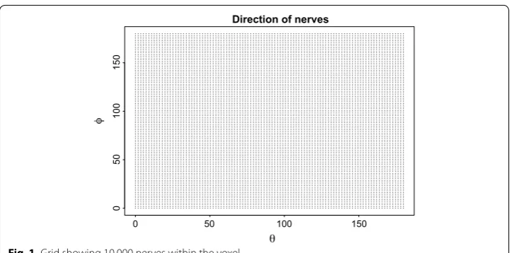
The method of representing the direction of nerves in a voxel can be represented by points on the surface of a sphere of unit radius, without the loss of generality. This means that the parameters θ and φ for any nerve are contained within the intervals (0◦, 180◦)
and (0◦, 360◦) , respectively. Furthermore in this scenario, diametrically opposite points
are equivalent, so it suffices to work on a hemisphere. This translates to φ being
con-tained in an interval (0◦, 180◦) . Since, the number of nerve fibers, K, within a voxel is unknown, it is chosen to (severely) overestimate the number of nerves and obtain their directions by subdividing these intervals into roughly one hundred equal parts. Thereby, a grid with each point representing a unique nerve within the voxel is obtained. This is shown in Fig. 1.
Performing the regression
Now that it is possible to compute M, regression analysis can be performed. Given that
the model has been over-parameterized, it is important to remove all nerves that do not have a contribution. This is achieved by using a form of regularized linear regression called elastic net [22]. In classical regression, the estimate for f is obtained by minimiz-ing the followminimiz-ing function:
(3)
M=
e−b1d e−b1dr1tg(θ1,φ1)r1 . . . e−b1dr1tg(θK,φK)r1 e−b2d e−b2dr2tg(θ1,φ1)r2 . . . e−b2dr2tg(θK,φK)r2
. .
. ... ...
e−bnd e−bndrntg(θ1,φ1)rn . . . e−bndrtng(θK,φK)rn
.
(4) y=Mf+ǫ
In contrast, elastic net regularization adds a penalty term with the function in Eq. 6 being minimized.
The reason classical least-squares regression is not employed is that there is no variable selection or shrinkage performed in the operation, and performing stepwise selection process would be computationally expensive. The adoption of elastic net regularization
within this method allows variable selection for d and K, which is necessary to run the
proposed efficient algorithm. If existing methods were employed, the classical least-squares regression would inhibit the reasonable selection of d and K.
Processing the output
In Eq. 6 when α is set to 1, a strenuous variable selection process is implemented. This
can potentially cause the model to be under-identified, meaning that some, or all, nerve
contributions cannot be accounted for in the signals. On the other hand, setting α to 0
causes too many nerves to be represented. Given this sensitivity, α is chosen closer to 0
to prevent potential underdetection of nerves. This leads to each true nerve being over-estimated by a group of closely-related nerves. Therefore, to further reduce the number of nerves to a plausible number, clustering is performed. Partitioning around mediods (pam) is performed based on a dissimilarity matrix using an adjusted angular distance, the need for which arises due to the axial nature of the data.
where ω(v,w)=cos−1 v·w
||v||2||w||2
and v,w∈Rk.
Algorithm
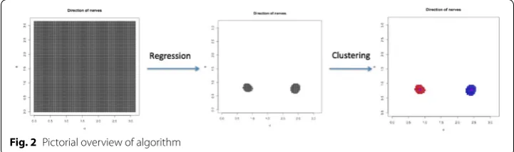
The overview of the steps used for nerve estimation are shown in Alg. 1 and a pictorial
overview is shown in Fig. 2. If existing methods for resolving intravoxel white matter
were employed, values of d and K could not be determined. Steps 1 and 2 of the
algo-rithm require the flexibility of choosing values for these parameters. Thus, the elastic net is vital in ensuring this algorithm can run properly.
(6)
C(f)= ||y−Mf||22+(1−α)||f||1+α||f|| 2 2
(7) ωadj(·,·)=min(ω(·,·),π−ω(·,·)),
0 50 100 150
05
01
00
15
0
Direction of nerves
Algorithm 1 Algorithm for obtaining nerves through regression and cluster-ing
Require: {ri, bi, yi}n i=1
1: Select multiple plausible values ford
2: SelectK(ideally very large value)
3: Obtain set{(θj, φj)}Kj=1
4: ComputeM
5: Set α and perform elastic net regularized regression to obtain a sparse estimate for
volume fractions,f
6: Take all nerves with non-zero volume fractions and perform clustering to determine true number of nerves and their directions
Experimental results
Different experiments were performed to verify the accuracy of the proposed method. We consider only the undirected and attributed graph for all the experiments. All the
experiments are executed on 64 GB main memory in Intel Core i5 @ 3.70GHz on a
Win-dows 10 operating system. Python 2.7 is used to implement the algorithms with
net-workx package for graph related operations.
Experiments and results
The method’s performance was tested using multiple synthetic datasets. The datasets
included 64 diffusion gradients with bi=3000 for 1–3 nerve systems. Although the
model assumes additive Gaussian noise is added to the observations in Eq. 4, the data is
simulated using Rician noise to ensure positivity of signals. The procedure for obtaining noisy signal is shown in Eq. 8.
To account for the total amount of noise in the system, the signal-to-noise ratio (SNR) is defined by 1
σ . Nine datasets were simulated using Eq. 1 with S0=1 in conjunction wth
Eq. 8, one for each of 1-, 2-, and 3-nerve system at SNR = 30, 20, 10 (low, medium, high
noise). The true diffusivity was assumed to be d=0.001 mm2/s . To test the sensitivity of the diffusivity parameter, three dictionaries were created with different diffusivity values: d=0.005 , d=0.001 , and d=0.002 . These correspond to 50% of true value, 100% of
(8) yi=
µi S0 +ǫi,1
2
true value, and 200% of true value. It should also be noted that the lowest and highest chosen values form a reasonable range for apparent diffusivity in the human brain.
Tables 1, 2, and 3 present the nerve direction estimation for 1-, 2-, and 3-nerve sys-tems, respectively. To summarize the precision of the estimated directions in relation to
the true values, the adjusted angular deviation was calculated by using Eq. 7.
Further-more, a mean angular deviation is also presented for multi-nerve systems. It should also be noted that the α-value for elastic net (Eq. 6) was set to 0.2 except in the 3-nerve
sys-tem at SNR = 10 where it was set to 0, and 1-, 2-nerve syssys-tems with d=0.0005 where
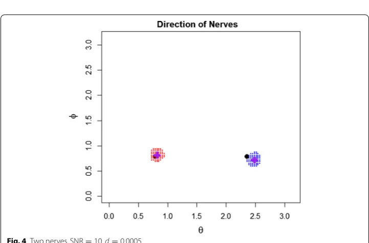
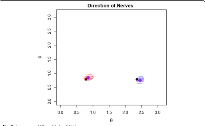
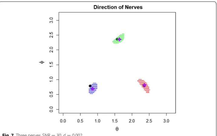
it was set to 1. Given the large number of experiments, Figs. 3, 4, 5, 6 and 7 present a graphical view of the estimation corresponding to the bolded lines in Tables 1, 2, and 3.
Table 1 Estimation results for 1-nerve {(45, 45)}
ED: estimated direction; AAD: adjusted angular distance
SNR d=0.0005 d=0.001 d=0.002
ED AAD ED AAD ED AAD
30 (120.6, 109.8) 84.21 (46.8, 45.0) 1.80 (48.6, 46.8) 3.83
20 (46.8, 46.8) 2.22 (46.8, 46.8) 2.22 (45.0, 46.8) 1.27
10 ( 46.8, 43.2) 2.22 ( 46.8, 43.2) 2.22 ( 45.0, 41.4) 2.55
Table 2 Estimation results for 2-nerves {(45, 45),(135, 45)}
ED: estimated direction; AAD: adjusted angular distance
SNR d=0.0005 d=0.001 d=0.002
ED AAD Mean AAD ED AAD Mean AAD ED AAD Mean AAD
30 (48.6, 46.8) 3.83 3.715 (48.6, 45.0) 3.60 3.600 (48.6, 46.8) 3.83 2.550
(138.6, 45.0) 3.60 (138.6, 45.0) 3.60 (135.0, 43.2) 1.27
20 (48.5, 45.0) 3.50 4.515 (48.6, 41.4) 4.45 5.185 (48.6, 41.4) 4.45 5.875
(140.4, 46.8) 5.53 (140.4, 48.6) 5.92 (142.2, 46.8) 7.30
10 ( 46.8, 46.8) 2.22 4.900 ( 46.8, 46.8) 2.22 4.760 ( 48.6, 48.6) 4.45 4.990
( 142.2, 41.4) 7.58 ( 142.2, 43.2) 7.30 ( 140.4, 43.2) 5.53
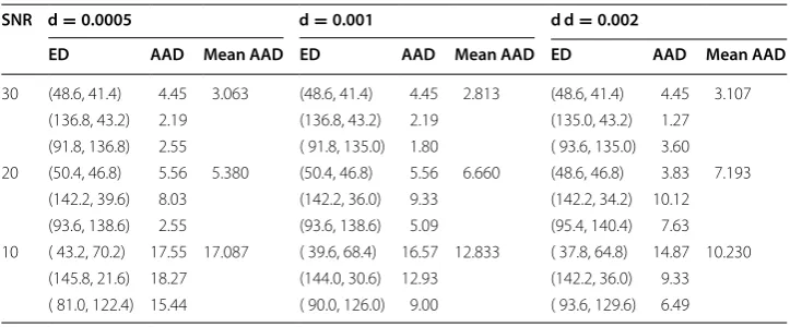
Table 3 Estimation results for 3-nerves {(45, 45),(135, 45),(90, 135)}
ED: estimated direction; AAD: adjusted angular distance
SNR d=0.0005 d=0.001 d d=0.002
ED AAD Mean AAD ED AAD Mean AAD ED AAD Mean AAD
30 (48.6, 41.4) 4.45 3.063 (48.6, 41.4) 4.45 2.813 (48.6, 41.4) 4.45 3.107
(136.8, 43.2) 2.19 (136.8, 43.2) 2.19 (135.0, 43.2) 1.27
(91.8, 136.8) 2.55 ( 91.8, 135.0) 1.80 ( 93.6, 135.0) 3.60
20 (50.4, 46.8) 5.56 5.380 (50.4, 46.8) 5.56 6.660 (48.6, 46.8) 3.83 7.193
(142.2, 39.6) 8.03 (142.2, 36.0) 9.33 (142.2, 34.2) 10.12
(93.6, 138.6) 2.55 (93.6, 138.6) 5.09 (95.4, 140.4) 7.63
10 ( 43.2, 70.2) 17.55 17.087 ( 39.6, 68.4) 16.57 12.833 ( 37.8, 64.8) 14.87 10.230
(145.8, 21.6) 18.27 (144.0, 30.6) 12.93 (142.2, 36.0) 9.33
Discussion
The proposed method utilizes regularized regression and clustering techniques for estimation of the principal direction of nerves within a voxel. The method’s robustness
has been heavily relied on because the apparent diffusivity, d, for the voxel is crudely
picked from a plausible range. A test for sensitivity shows that the method’s performance is mostly unaffected when this parameter is obtained within a reasonable range of the
true value. In the event that d is severely underestimated, the number of nerves can be
overestimated, since some of the artificial nerves do not get eliminated by the regression 0.0 0.5 1.0 1.5 2.0 2.5 3.0
0.
00
.5
1.
01
.5
2.
02
.5
3.
0
Direction of nerves
θ
φ
Fig. 3 One nerve, SNR=10 , d=0.001
step. This is explained by the inability of the system to produce higher dampening effects with little diffusivity and a small number of nerves. On the other hand, a severe
overesti-mation in d can cause an underestimation of nerves because their corresponding
damp-ening effects are exceedingly pronounced. In the case of 1-, 2-nerve systems at SNR=30
with d=0.0005 , α (Eq. 6) had to be set equal to 1 to reduce overestimation of nerves. Alternatively in the future, it is possible to devise algorithms that learn d simultaneous to the regression. It is also possible to borrow information from other relevant algorithms
or perform additional MRI-related experiments to obtain an estimated value of d, which
Fig. 5 Two nerves, SNR=10 , d=0.002
0.0 0.5 1.0 1.5 2.0 2.5 3.0
0.
00
.5
1.
01
.5
2.
02
.5
3.
0
Direction of nerves
θ
φ
would then reduce the onus of estimation off the assumptions of this model and make it easier to pick more lenient values for regularization.
It should also be noted that in the case of 3-nerve systems at SNR=10 , the α-value
had to be dropped to 0 exactly. This is explained by the complexity of the confounded dampening effect from the three nerves and high-noise. This issue is slightly harder to overcome, but it is argued that a finer discretization of the parameter space may poten-tially provide a solution and even improve estimation accuracy.
Figures 3, 4, 5, 6 and 7 show that the number of clusters formed were obvious. This may not be the case in the future. Therefore, it would be advisable to run the clustering algorithm multiple times with a variable number of clusters, and, additionally, use an external criteria (such as the elbow method using sum of squared errors) to evaluate the best number of nerves.
The adoption of elastic net regularization enables variable selection for the proposed method. Given a sensible interval for the diffusivity parameter and a severe overestimate
for the number of nerves, the selection for d and K are reasonable and can be used in the
algorithm. This is computationally more efficient than running a Bayesian and collabora-tive approach to estimate these variables.
Conclusion and future work
The proposed method has shown promising preliminary results in a host of unfavora-ble conditions, including noisy data and imprecision in parameter assumptions. In the future, the method’s efficacy will be tested on real patient data along with a presentation of comparative analyses with other relevant methods in the field.
Abbrevations
Acknowledgements
We sincerely and gratefully acknowledge the following organizations for their help and support: Department of Defense for funding the AEOP UNITE participants as well as computing facilities via Grants #W911NF‑16‑1‑0416 and #W911NF‑17‑1‑0088. National Science Foundation for funding the RET participants via #1710716 as well as computing facilities via Grant #1625677.
Authors’ contributions
All authors have contributed to the research and manuscript with the order they appear. All authors discussed the final results as well as improved the final manuscript. All authors read and approved the final manuscript.
Funding
This research was funded by the Army Education Outreach Program (AEOP) UNITE and National Science Foundation Research Experience for Teachers (RET) program.
Availability of data and materials
This research analyzed experimental data that was created by the authors to reflect realistic parameters and variation between individual brains. The analysis was conducted in R.
Competing interests
The authors declare that they have no competing interests. Author details
1 Army Education Outreach Program UNITE, Las Vegas, USA. 2 National Science Foundation Research Experiences for Teachers Program, Las Vegas, USA. 3 University of Nevada, Las Vegas, Las Vegas, USA.
Received: 27 April 2019 Accepted: 25 June 2019
References
1. Bloomington IU. Grey matter and white matter. Bloomington: Indiana University; 2003. 2. Swan J. Spinal notes. The University of New Mexico—Class Notes; 2005.
3. Graham R, McCabe H, Sheridan S. Neural networks for real‑time pathfinding in computer games. ITB J. 2004;5(1):21. 4. Bansal R, Hao X, Liu F, Xu D, Liu J, Peterson BS. The effects of changing water content, relaxation times, and tis‑
sue contrast on tissue segmentation and measures of cortical anatomy in mr images. Magn Reson Imaging. 2013;31(10):1709–30.
5. Johansen‑Berg H, Behrens TE. Diffusion mri: from quantitative measurement to in‑vivo neuroanatomy, vol. 2. Cam‑ bridge: Academic Press; 2009.
6. Lenglet C, Deriche R, Faugeras O. Inferring white matter geometry from diffusion tensor mri: application to con‑ nectivity mapping. In: European conference on computer vision. Springer, 2004, pp. 127–140.
7. Jones DK, Knosche TR, Turner R. White matter integrity, fiber count, and other fallacies: the do’s and don’ts of diffu‑ sion mri. Neuroimage. 2013;73:239–54.
8. Vos SB, Jones DK, Jeurissen B, Viergever MA, Leemans A. The influence of complex white matter architecture on the mean diffusivity in diffusion tensor mri of the human brain. Neuroimage. 2012;59(3):2208–16.
9. Behrens TE, Berg HJ, Jbabdi S, Rushworth MF, Woolrich MW. Probabilistic diffusion tractography with multiple fibre ori‑ entations: what can we gain? Neuroimage. 2007;34(1):144–55.
10. Pisharady PK, Sotiropoulos SN, Duarte‑Carvajalino JM, Sapiro G, Lenglet C. Estimation of white matter fiber parame‑ ters from compressed multiresolution diffusion MRI using sparse bayesian learning. Neuroimage. 2018;167:488–503. 11. Tuch DS, Reese TG, Wiegell MR, Makris N, Belliveau JW, Wedeen VJ. High angular resolution diffusion imaging reveals
intravoxel white matter fiber heterogeneity. Magn Reson Med. 2002;48(4):577–82.
12. Anderson AW. Measurement of fiber orientation distributions using high angular resolution diffusion imaging. Magn Reson Med. 2005;54(5):1194–206.
13. Kaden E, Knosche TR, Anwander A. Parametric spherical deconvolution: inferring anatomical connectivity using diffusion mr imaging. Neuroimage. 2007;37(2):474–88.
14. Sotiropoulos SN, Bai L, Morgan PS, Auer DP, Constan‑tinescu CS, Tench CR. A regularized two‑tensor model fit to low angular resolution diffusion images using basis directions. J Magn Reson Imaging. 2008;28(1):199–209.
15. Sotiropoulos SN, Jbabdi S, Andersson JL, Woolrich MW, Ugurbil K, Behrens TE. Rubix: combining spatial resolutions for bayesian inference of crossing fibers in diffusion mri. IEEE Trans Med Imaging. 2013;32(6):969–82.
16. Coupe P, Manjon JV, Chamberland M, Descoteaux M, Hiba B. Collaborative patch‑based super‑resolution for diffusion‑weighted images. Neuroimage. 2013;83:245–61.
17. Scherrer B, Schwartzman A, Taquet M, Sahin M, Prabhu SP, Warfield SK. Characterizing brain tissue by assessment of the distribution of anisotropic microstructural environments in diffusion‑compartment imaging (diamond). Magn Reson Med. 2016;76(3):963–77.
18. Tournier JD, Calamante F, Gadian DG, Connelly A. Direct estimation of the fiber orientation density function from diffusion‑weighted mri data using spherical deconvolution. Neuroimage. 2004;23(3):1176–85.
19. Ozarslan E, Shepherd TM, Vemuri BC, Blackband SJ, Mareci TH. Resolution of complex tissue microarchitecture using the diffusion orientation transform (dot). Neuroimage. 2006;31(3):1086–103.
21. Aganj I, Lenglet C, Sapiro G, Yacoub E, Ugurbil K, Harel N. Reconstruction of the orientation distribution function in single‑and multiple‑shell q‑ball imaging within constant solid angle. Magn Reson Med. 2010;64(2):554–66. 22. Zou H, Hastie T. Regularization and variable selection via the elastic net. J R Stat Soc Series B Stat Methodol.
2005;67(2):301–20.
23. Chiu C, Zhan J. Deep learning for link prediction in dynamic networks using weak estimators. IEEE Access. 2018;6(1):35937–45.
24. Bhaduri M, Zhan J. Using empirical recurrences rates ratio for time series data similarity. IEEE Access. 2018;6(1):30855–64.
25. Wu J, Zhan J, Chobe S. Mining association rules for low frequency itemsets. PLoS ONE. 2018;13(7):e0198066. 26. Ezatpoor P, Zhan J, Wu J, Chiu C. Finding top‑k dominance on incomplete big data using mapreduce framework.
IEEE Access. 2018;6(1):7872–87.
27. Chopade P, Zhan J. Towards a framework for community detection in large networks using game‑theoretic mod‑ eling. IEEE Trans Big Data. 2017;3(3):276–88.
28. Bhaduri M, Zhan J, Chiu C. A weak estimator for dynamic systems. IEEE Access. 2017;5(1):27354–65.
29. Bhaduri M, Zhan J, Chiu C, Zhan F. A novel online and non‑parametric approach for drift detection in big data. IEEE Access. 2017;5(1):15883–92.
30. Chiu C, Zhan J, Zhan F. Uncovering suspicious activity from partially paired and incomplete multimodal data. IEEE Access. 2017;5(1):13689–98.
31. Ahn R, Zhan J. Using proxies for node immunization identification on large graphs. IEEE Access. 2017;5(1):13046–53. 32. Zhan F, Waters B, Mijangos M, Chung L, Bhagat R, Bhagat T, Pirouz M, Chiu C, Tayeb S, Ploutz E, Zhan J, Gewali L. An
efficient alternative to personalized page rank for friend recommendations. In: The 15th IEEE annual consumer com‑ munications and networking conference, January 12–15. USA: Las Vegas; 2018.
33. Zhan F, Laines G, Deniz S, Paliskara S, Ochoa I, Guerra I, Tayeb S, Chiu C, Pirouz M, Ploutz E, Zhan J, Gewali L, Oh P. Prediction of online social networks users’ behaviors with a game theoretic approach. In: The 15th IEEE annual consumer communications and networking conference, January 12–15. USA: Las Vegas; 2018.
Publisher’s Note