© Universiti Tun Hussein Onn Malaysia Publisher’s Office
IJIE
Journal homepage: http://penerbit.uthm.edu.my/ojs/index.php/ijie
The International
Journal of
Integrated
Engineering
ISSN : 2229-838X e-ISSN : 2600-7916
Classification of Corneal Nerve Images
u
sing Machine
Learning Techniques
Tooba Salahuddin
1, Uvais Qidwai
1*1Department of Computer Science and Engineering , College of Engineering, Qatar University, Doha, QATAR
*Corresponding Author
DOI: https://doi.org/10.30880/ijie.2019.11.03.001
Received 18 February 2019; Accepted 3 July 2019; Available online 3 September 2019
1. Introduction
A debilitating co mplication of many chronic diseases is neuropathy. It is a disorder of the central nervous system which degrades the quality of life o f the patient. Early and time ly diagnosis of neuropathy is beneficial in many ways. It can help determine the severity level of nerve da mage and a llo w the monitoring of disease growth. Pe riphera l neuropathy is distinguished by numbness in the limbs and is the most prevalent co mplication of d iabetes. Other visib le effects of neuropathy include foot ulceration [1]. One of the earliest hidden symptoms of neuropathy is small fiber nerve damage and is apparent in a very early stage prior to the occurren ce of visible symptoms [2]. On the other hand, visible sy mptoms of neuropathy occur only when the da mage has reached the long nerve fibers. There fore, prec ise and prompt diagnosis of neuropathy is necessary for prognosis, early recognition of subclin ical neuropathy, monitoring disease growth, classifying disease severity and suggesting relevant therapy plans [3].
State-of-the-art techniques for detecting nerve da mage inc lude electrophysiology, quantitative sensory testing, skin biopsy and nerve conduction studies. Most of these techniques are unable to detect small nerve fiber loss and provide subjective and inaccurate results [4]. A lthough skin biopsy has been successful in detecting small nerve fiber loss, the technique itself is invasive and therefore cannot be conducted frequently. Moreover, it is time consuming and requires expert skill [5].
Recently, in vivo corneal confocal microscopy (CCM) has e merged as a non -invasive, objective surrogate and imaging bio marker for detecting nerve fiber defic its. Due to the scientific fact that sma ll nerve fibers are present in the human cornea, an insight into the subbasal nerve ple xus of the cornea can detect very early neuropathy. The
Abstrac t: Recent research shows that small nerve fiber da mage is an ea rly detector of neuropathy. These small nerve fibers are present in the hu man cornea and can be visualized through the use of a corneal confocal microscope. A series of images can be acquired fro m the subbasal nerve ple xus of the cornea. Befo re the images can be quantified for nerve loss, a hu man e xpe rt manually traces the nerves in the image and then classifies the image as having neuropathy or not. So me nerve trac ing algorith ms are availab le in the literature, but none of the m are reported as being used in c lin ical practice. An alte rnate practice is to visually c lassify the image for neuropathy without quantification. In this paper, we evaluate the potential of various mach ine learn ing techniques for automating corneal nerve image classificat ion. First, the images are down-sa mpled using discrete wavelet transform, filtering and a number of morphologica l operations. The resulting b inary image is used for e xt racting characteristic features of the image. Th is is follo wed by train ing the clas sifier on the e xtracted features. The tra ined classifier is then used for pred icting the state of the nerves in the images. Our e xpe riments yield a classification accuracy of 0.91 reflecting the effectiveness of the proposed method.
transparency of the epitheliu m enables the laser to penetrate into the different layers of the cornea and give a clear visualizat ion. Thus, CCM images reveal a detailed and magnified structure of the densely innervated cornea of the human eye.
Studies have demonstrated the effectiveness and reproducibility of CCM in detecting neuropathy in diabetic patients [3] and subjects with Parkinson’s disease [6], Multip le Sclerosis [7], chronic migraine [8], chemotherapy induced neuropathy [9], human immunodeficiency virus [10] and acute ischemic stroke [11].
CCM p rovides a detailed and magnified visual representation of the corneal nerve structure. Current limitations of such a pro mising tool inc lude the tedious process of manual nerve tracing by c linic ians for nerve para meter quantification and classification of images to define the degree of nerve damage. Rapid, accurate and automated quantification of CCM images by explo iting image processing techniques tends to be a challenging task. Nevertheless, significant research has been conducted in this domain [12]–[17] atte mpting to address the challenge by employing different techniques.
To the best of our knowledge, currently there is no fully auto matic system for classificat ion of CCM images captured from the sub-basal nerve ple xus of the cornea. One research group [18] has proposed the idea of neuropathy classification through convolutional neural networks, but it is a pilot study and lacks an in -depth analysis of the results.
Therefore, the primary contribution of this research is to evaluate machine lea rning techniques for classifying corneal nerve images, using adaptive neuro fu zzy in ference system (ANFIS), support vector mach ines (SVM ), naïve Bayes (NB), linear discriminant analysis (LDA ), classification trees and k-nearest neighbours (KNN). The classifie r can distinguish between the state of nerves in the corneal images as normal or abnormal. The proposed system significantly speeds up the classification process which allows for early diagnosis of neuropathy .
This paper is organized as follows. The subsequent section presents related work on CCM image segmentation and classification. Th is is followed by a detailed description of the proposed method including nerve segmentation a long with a description of machine learn ing algorith ms in Section III. The evaluation of the c lassification technique is reported in Section IV which e xp lains the e xperimental setting and achieved results. Finally, Section V concludes the paper with possible future research directions .
2.
Related Work
A factor hindering the advancement of CCM for neuropathy detection is the absence of precise and automated systems for image analysis and disease prediction. Precise nerve seg mentation and quantification techniques are required for the establishment of reliable and consistent standards for nerve measurements. Researchers have approached nerve segmentation of CCM images using various methods. Ruggeri et a l. [17] p roposed a nerve recognition and tracing method based on vessel segmentation in ret inal images [15]. Th is method starts with fixed locations for seed point e xt raction and trac ks nerve p ixe ls by e xpanding the region of interest. Conflicts at nerve intersections are rectified by using a technique called bubble analysis wh ich identifies nerve pixe ls by going through concentric c irc les fro m the center point. Then, fuzzy k-means clustering is applied to classify pixe ls as nerve or non-nerve. The proposed algorith m was eva luated on 12 CCM images captured fro m a sit -la mp CCM. The algorith m showed a tendency for increased fa lse positives, possibly due to the e xistence of other structures in the bac kground. The segmentation time per image was 4 – 5 minutes. The same a lgorith m was modified by Scarpa et a l. [16] to include the use of Gabor filters before nerve tracking. A further enhancement of the algorithm was performed by Po letti and Ruggeri [14], by allo wing mult iple orientations of the lines for seed points extraction. The algorith m was tested on 30 corneal nerve images and the segmentation time was reduced to 25 secon ds per image.
Dabbah et al. [19] developed a dual model a lgorith m for nerve segmentation by applying Gabor and Gaussian filters. A co mparative ana lysis of the proposed algorithm with another previously reported method for detecting asbestos fibers [20] showed improved performance for the dual model approach. Later, the method was modified with mu ltiscale enhancement in [21], and p ixe l classification was approached through neural networks and random forest classifiers. In another study [22], c lassification was performed using SVM . A l-Fahdawi et a l. [12] approached nerve segmentation through morphologica l operations. They applied coherence and Gaussian filte rs for contrast enhancement followed by dilation and erosion operations for noise reduction. Canny edge detection is employed for detecting nerve edges. The algorithm required about 7 seconds per image and was tested on approximately 1500 images.
The authors also used U-Net for neuropathy classification of images. They tested the trained model on 100 images and obtained an accuracy of 83% fo r binary classification (healthy/pathological). No further details on the experimental results were provided.
In summa ry, the re lated research focusses on the segmentation techniques for CCM images and the doma in o f neuropathy classification of CCM images is yet to be explo red. We show the potential of machine learning techniques for automatic classification of CCM images. In the following sections, we discuss our methodology.
3.
Materials and Methods
3.1
Dataset
The performance of the c lassifier was evaluated on 297 CCM images taken fro m the dataset in [25]. 93 images belong to the norma l class, while the rest belong to the abnorma l class. The images were captured using a laser scanning corneal confocal microscope, Heide lberg Retina l To mograph, equipped with Rostock Corneal Module (HRT -RCM: He idelberg Engineering, He idelberg, Germany). The images are of size 384x384 pixe ls and saved in JPG format.
3.2
Nerve Segmentation
During nerve segmentation, the images first undergo discrete wavelet transform to reduce the size o f the image to one-fourth of the original. For the elimination of background noise and enhancement of linear structures Gaussian and coherence filters are applied. The diffusion scheme for coherence filter was chosen to be optimized derivative ke rnels, because it gave the best results. The resultant image is passed through a Gaussian filter with a variance of 0.5. this is followed by binarizat ion with a threshold of 0.35. A number of morphologica l operations are applied to the binarized image to re move further noise and link b roken segments. The final step is skeletonization wh ich reduces the detected nerves to one-pixel wide segments. Further details on the image segmentation process are described in [26].
Fig. 1. Nerve segmentation outputs (a) original CCM image, (b) discrete wavelet transform, (c) coherence and gaussian filter output, (d) binary image, (e) skeleton image, (f) final segmented image
3.3
Feature Extraction
In this step, features representing the image are extracted from the binary segmented nerve image. We extracted three features for each image:
1) Total nerve fiber length (NFL) calculated as summation of all nerve pixels, 2) Entropy of the image, and
3) Area occupied by the nerves .
(a) (b) (c)
3.4
Machine Learning
This section briefly explains the machine learning algorithms used in this study.
3.4.1
Adaptive Neuro Fuzzy Inference System
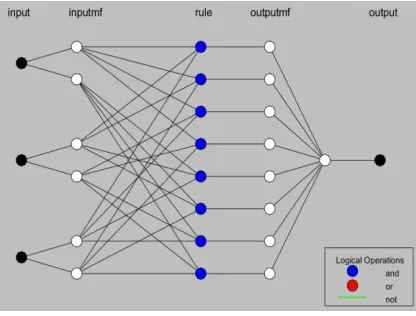
ANFIS is a mach ine learn ing algorithm wh ich comb ines the learning power of fuzzy inference systems and artific ial neura l networks into a robust framework [27]. It consists of five layers. In the first layer, the me mbership functions specify the me mbe rship degree of each input variab le. These me mbership functions are formulated during the training phase. Using these me mbership functions, ANFIS creates a fu zzy inference system (FIS) wh ich map the inputs to their corresponding outputs. The inferences from the ru le base are used in the second and fourth layer to adjust the firing strength of each rule. The fourth layer generates the outputs using a linear polynomial equation. The last layer concatenates all outputs into a single output.
A two-pass learning algorithm is imp le mented during the lea rn ing stage [28]. The forward pass consists of updating the parameters using least squares estimation to produce the output. During the backward pass, error is computed across all layers and parameter values are updated accordingly using gradient descent algorithm.
The ANFIS network builds a FIS fro m the three input features, mapping the m to the output using the me mbership functions. Hence, the FIS is tra ined on the randomly selected training data. The architecture of the ANFIS network is displayed in Fig. 2. The figure shows only four layers because the second and third layers are displayed as one, name ly the rule layer.
Fig. 2. Architecture of ANFIS
3.4.2
Support Vector Machine
SVMs are known as univers al lea rners because they usually perform we ll in most classification proble ms. SVM aims to create an optimal hyperplane with ma ximu m marg in, that separates the two classes of data. The points closest to the hyperplane are called support vectors, and they d etermine the position of the hyperplane. Consider a set of train ing
samples, , each having a label fro m a set or labels, . The SVM classifie r creates a classifier of the form [29]:
,
(1)
Where belongs to a set of real constants, is the bias and is a kerne l function. Co mmonly used kernel functions
are: linear , polynomial with degree d , and radial basis function .
The lines that separate the data are defined by:
(2)
(3)
This is equivalent to the non-linear function:
(4)
3.4.3
Naïve Bayes
Naïve Bayes is a simp le probabilistic classificat ion algorithm that classifies based on the like lihood of occurrence [30]. It assumes that features are independent given the class. During train ing, probabilit ies are ca lculated for each feature value given a class label. These probabilities are used to predict the label of a test sample.
Consider a feature vector, , where each feature value is ta ken fro m a distribution . The set
omega contains all feature vectors: . Let be the class label of an example.
The class posterior probabilities given a feature vector can be defined as a discriminant function:
. This can be rewritten after applying Bayes rule:
(5)
.
Here, is the sa me for all class es and can be eliminated. Thus, Bayes discriminant functions can be written
as the following: , where is termed as the class
-conditional probability distribution.
Finally, the Bayes classifier can be defined as:
(6)
finds the ma ximu m a posteriori probability for any e xa mp le x. Extending this to simplified naïve Bayes assumption that features are independent given class, we get the following form:
(7)
3.4.4
K-Nearest Neighbors
One of the c lassical and simp lest nonparametric c lassification a lgorith ms is the k -nearest neighbor (KNN) c lassifier, which c lassifies new e xa mp les based on nearest sample observation. It is based on the assumption that when feature vectors for training data points are projected into a subspace, any new data point can be classified based on its proximity to its k nearest neighbors [31].
Consider a set of tra ining samples, , each having a labe l fro m a set or labels, , and features. The feature vector for is represented as . A new sa mple is assigned label if a ma jority
of nearest neighbors of possess the label .
Nearness can be measured using any of the several distance measures. The most common ones are Euclidean distance (L2 norm), Manhattan distance (L1 norm) or Max norm.
The Euclidean distance between two samples and is defined as:
(8)
The number of nearest neighbors in the neighborhood, k, is usually tuned as a hyperpara meter. Emp irica lly, as k increases, the accuracy of the prediction decreases.
Several variat ions of KNN e xist in the literature. Weighted KNN adds weight to the vote of each label in the neighborhood based on its distance from the test sample [32]. Epsilon-ball KNN is a method that selects neighbors within a distance from the test s ample.
3.4.5
Classification Trees
Classification trees split the training data into partitions, based on mapping of inputs to the outputs. Thus, by creating partitions it learns the diffe rent patterns occurring in the data. Co mmonly used split criteria inc lude gini inde x , informat ion gain and entropy. Partit ioning the data results in the c reation of a tree, where the root of the tree is one feature value, and subsequent nodes are other feature values. Each level contains feature values corresponding to one feature. The leaf nodes predict the class of a given sample. As the tree goes deeper, the learning represents overfitting. Consequently, pruning the tree to a certain depth is a tunable hyperparameter.
3.4.6
Linear Discriminant Analysis
two categories and minimize the variat ion within each category. The c lass of a test sample is predicted using Bayes’ Theorem as explained in Section 3.4.3.
4.
Experiments and Results
4.1
Experimental Setting
All imple mentation was done using MATLAB. In the preprocessing stage, data are normalized by dividing each value by the ma ximu m of its colu mn. Data is randomly selected for train ing and testing using a ratio of 3:2 for train and test sets. For generating an initia l FIS, the grid partit ioning method is used. ANFIS is trained on the initia l FIS for 30 training epochs. The trained FIS is used to calculate the training error and trained repeatedly to generate the best FIS. The FIS with the highest accuracy is selected as the best one.
Besides ANFIS, classifiers are also trained using Support Vector Machines (SVM), Naïve Baiyes (NB), linear discriminant analysis (LDA), c lassification trees (Tree) and k-nearest neighbors (KNN). For SVM , a linear kernel with a scale of 1 was used. Sequential mo mentum optimizer (SM O) was used as the optimizat ion method which uses second order polynomial informat ion to speedup convergence. The model identified 42 support vectors from the training data. The kernel smoothing type for NB was tuned to be Gaussian which is defined by the following formula:
(9)
The number of nearest neighbors in KNN was set to 5 and Euclidean distance was used to determine nearness between the samples. The same train and test subsets are used for all. For a ll models, hyperparameters were optimized to give the best results.
4.2
Performance Measures
The following performance measures are used in this study to evaluate the re sults of the ANFIS classifier:
In this study, the performance measures of accuracy, precision, recall and macro F1were used to evaluate the performance. Accuracy is defined as TP+TN/TP+TN+FP+FN, prec ision as TP/TP+FP and recall as TP/TP+FN, where TP stands for true positives, FP for fa lse positives, TN for true negatives and FN for fa lse negatives. Macro F1 is the harmonic mean of precision and recall.
4.3
Results and Discussion
The predicted values by ANFIS are scaled to confine between the range [0,1] using the following equation.
(10)
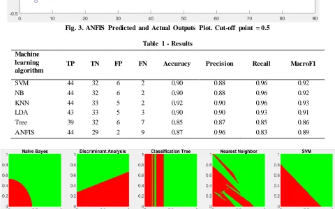
where yi is the predicted ANFIS output for the ith data point. Fig. 3 compares the actual output and the predicted output
by ANFIS on the testing data. Tuples (data points) fro m the testing data are represented by the x-a xis (84 tuples). The y-axis shows the actual and scaled predicted output for each tuple. For e xa mple , for the second data point, the actual output, y3, is 1, and the scaled predicted output, ys3, is 0.98 (almost 1).
After calculating the scaled predicted output, the most satisfying range for each class is selected. The highest accuracy for this experiment is acquired given by the rule:
IF ysi > 0.8 THEN ysi = 1 ELSE ysi = 0,
where class ‘normal’=0, ‘abnormal’=1, and the cutoff point is 0.5. Hence, the ranges for class 1 and class 0 are (0.5,1] and [0,0.5] respectively. The cutoff line is shown in Fig. 4 as a dotted line where Y=0.5. For e xa mple, for the first data point, the actual output, y2=1, and it coincides with the predicted output, ys2. Since the predicted output is greater than
0.5, thus, according to the rule, ys2=1, which makes it a true prediction.
the decision surfaces formed by all c lassifiers except ANFIS. Since it is a 2d plot, two features were considered for plotting the surface. The red region shows neuropathy while the green shows normal.
Fig. 3. ANFIS Predicted and Actual Outputs Plot. Cut-off point = 0.5
Table 1 - Results Machine
learning algorithm
TP TN FP FN Accuracy Precision Recall MacroF1
SVM 44 32 6 2 0.90 0.88 0.96 0.92
NB 44 32 6 2 0.90 0.88 0.96 0.92
KNN 44 33 5 2 0.92 0.90 0.96 0.93
LDA 43 33 5 3 0.90 0.90 0.93 0.91
Tree 39 32 6 7 0.85 0.87 0.85 0.86
ANFIS 44 29 2 9 0.87 0.96 0.83 0.89
Fig. 4 Decision surfaces formed by the classifiers
Since the classification relies heavily on the extraction of features from the images, which is preceded by the nerve segmentation procedure, classification accuracy can be increased by improving the segmentation output and extracting the right features. Performance can also be imp roved by extracting different kinds of features, and by combining clinica l features with the hand-crafted image features.
5.
Conclusion
We have presented an evaluation of six mach ine lea rning algorithms for the problem of neuropathy classification of corneal nerve images. In our e xperiments, we achieved the highest accuracy of 0.92 using the k-nearest neighbors algorith m. The automated process of classification solves the limitations posed by the current manual process. Further evaluations on other datasets are required to achieve better results. In future, we plan to continue our experiments and widen our research in this domain by e xtracting diffe rent kinds of features, incorporating deep learning, and observing the results on different kinds of datasets.
References
[1] C. Quattrini et al., “Surrogate markers of small fiber damage in human diabetic neuropathy,” Diabetes, 2007. [2] M. A. Dabbah, J. Graham, R. Malik, and N. Efron, “Detecting and Analyzing Linear Structures in Biomedical
Images: A Case Study Using Corneal Nerve Fibers,” in Medical Image Processing, 2011.
Neurologic Disease,” Invest. Ophthalmol. Vis. Sci., vol. 58, no. 9, pp. 3682–3682, 2017.
[4] P. Hossain, A. Sachdev, and R. A. Malik, “Early detection of diabetic peripheral neuropathy wit h corneal confocal microscopy,” Lancet. 2005.
[5] M. Brines et al., “Corneal nerve fiber size adds utility to the diagnosis and assessment of therapeutic response
in patients with small fiber neuropathy,” Sci. Rep., 2018.
[6] P. J. Podgorny, O. Suchowersky, K. G. Romanchuk, and T. E. Feasby, “Evidence for small fiber neuropathy in early Parkinson’s disease,” Park . Relat. Disord., 2016.
[7] J. Mikolajczak et al., “Patients with multiple sclerosis demonstrate reduced subbasal corneal nerve fibre
density,” Mult. Scler., 2017.
[8] R. Shetty, R. Deshmukh, R. Shroff, C. Dedhiya, and C. Jayadev, “Subbasal nerve plexus changes in chronic migraine,” Cornea, 2018.
[9] M. Ferdousi et al., “Corneal confocal microscopy detects small fibre neuropathy in patients with uppe r
gastrointestinal cancer and nerve regeneration in chemotherapy induced peripheral neuropathy,” PLoS One, 2015.
[10] H. I. Kemp et al., “Use of corneal confocal microscopy to evaluate small nerve fibers in patients with human
immunodeficiency virus,” JAMA Ophthalmol., 2017.
[11] A. Khan et al., “Corneal confocal microscopy detects corneal nerve damage in patients admitted with acute
ischemic stroke,” Strok e, 2017.
[12] S. Al-Fahdawi et al., “A fully automatic nerve segmentation and morphometric parameter q uantification system
for early diagnosis of diabetic neuropathy in corneal images,” Comput. Methods Programs Biomed., 2016. [13] R. A. Dabbah, M. A., Graham, J., Tavakoli, M., Petropoulos, Y., & Malik, “Nerve fibre extraction in confocal
corneal microscopy images for human diabetic neuropathy detection using gabor filters,” Med. Image Underst. Anal., vol. 254–258, 2009.
[14] E. Poletti and A. Ruggeri, “Automatic nerve tracking in confocal images of corneal subbasal epithelium,” in
Computer-Based Medical Systems (CBMS), 2013 IEEE 26th International Symposium, 2013, pp. 119–124. [15] A. Grisan, E., Pesce, A., Giani, A., Foracchia, M., & Ruggeri, “A new tracking system for the robust extraction
of retinal vessel structure,” in Engineering in Medicine and Biology Society, 2004. IEMBS’04. 26th Annual International Conference of the IEEE, p. Vol. 1, pp. 1620–1623.
[16] F. Scarpa, E. Grisan, and A. Ruggeri, “Automatic recognition of corneal nerve structures in images from confocal microscopy,” Investig. Ophthalmol. Vis. Sci., 2008.
[17] A. Ruggeri, F. Scarpa, and E. Grisan, “Analysis of corneal images for the recognition of nerve structures,” in
Engineering in Medicine and Biology Society, 2006. EMBS’06. 28th Annual International Conference of the IEEE, 2006, vol. 4739–4742.
[18] A. Colonna, F. Scarpa, and A. Ruggeri, “Segmentation of Corneal Nerves Using a U-Net-Based Convolutional Neural Network,” 2018, pp. 185–192.
[19] M. A. Dabbah, J. Graham, I. Petropoulos, M. Tavakoli, and R. A. Malik, “Dual-model automatic detection of nerve-fibres in corneal confocal microscopy images,” in Lecture Notes in Computer Science (including subseries Lecture Notes in Artificial Intelligence and Lecture Notes in Bioinformatics), 2010.
[20] R. N. Dixon and C. J. Taylor, “Automated Asbestos Fiber Counting,” in 1979 Inst. Physics Conference, 1979. [21] M. A. Dabbah, J. Graham, I. N. Petropoulos, M. Tavakoli, and R. A. Malik, “Automatic analysis of diabetic
peripheral neuropathy using multi-scale quantitative morphology of nerve fibres in corneal confocal microscopy imaging,” Med. Image Anal., 2011.
[22] P. Guimaraes, J. Wigdahl, E. Poletti, and A. Ruggeri, “A fully-automatic fast segmentation of the sub-basal layer nerves in corneal images,” in 2014 36th Annual International Conference of the IEEE Engineering in Medicine and Biology Society, EMBC 2014, 2014.
[23] O. Ronneberger, P. Fischer, and T. Brox, “U-net: Convolutional networks for biomedical image segmentation,” in Lecture Notes in Computer Science (including subseries Lecture Notes in Artificial Intelligence and Lecture Notes in Bioinformatics), 2015.
[24] P. Guimarães, J. Wigdahl, and A. Ruggeri, “A Fast and Efficient Technique for the Automatic Tracing of Corneal Nerves in Confocal Microscopy,” Transl. Vis. Sci. Technol., 2016.
[25] I. Otel et al., “Diabetic peripheral neuropathy assessment through corneal nerve morphometry,” in Bioengineering (ENBENG), 2013 IEEE 3rd Portuguese Meeting, 2013.
[26] T. Salahuddin and U. Qidwai, “Neuro-Fuzzy Classifier for Corneal Nerve Images,” in IEEE-EMBS Conference on Biomedical Engineering and Sciences (IECBES), 2018, pp. 131–136.
[27] J. S. R. Jang, “ANFIS: Adaptive-Network-Based Fuzzy Inference System,” IEEE Trans. Syst. Man Cybern., 1993.
[28] N. Talpur, M. N. M. Salleh, and K. Hussain, “An investigation of membership functions on performance of ANFIS for solving classification problems,” in IOP Conference Series: Materials Science and Engineering, 2017.
1999.
[30] I. Rish, “An empirical study of the naive Bayes classifier,” in International Joint Conferences on Artificial Intelligence 2001 Work shop on Empirical Methods in Artificial Intelligence, 2001.