Multi-Input Multi-Output (MIMO) Control System with a State
Equation for Fusion Reactors
Yuya MIYOSHI and Yuichi OGAWA
Graduate School of Frontier Science, The University of Tokyo, Kashiwa 227-0882, Japan (Received 8 October 2013/Accepted 18 January 2014)
In future fusion reactors, plasma control can be anticipated to be quite complicated because actuators and diagnostics would be limited because of extreme environmental conditions, such as high neutron fluxes. In addition, control parameters and actuators are not in simple one-to-one correspondences (e.g., NBI power affects not only plasma current but also fusion power). This results in the need of using multi-input multi-output control systems. To confront this problem, we have developed a control system design that involves an state equation. In this research, simulations were performed in which three plasma parameters (fusion power, plasma current, and plasma density) were controlled using three actuators (NBI power, amount of gas puff, and inductively driven current). Parameters for these actuators were determined from the state equation, and the plasma parameters were simultaneously controlled with sufficiently high accuracy.
c
2014 The Japan Society of Plasma Science and Nuclear Fusion Research
Keywords: plasma control, PID theory, state equation, MIMO system, 0-D model DOI: 10.1585/pfr.9.1405015
1. Introduction
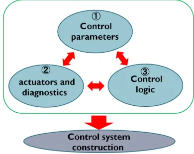
In designing DEMO or commercial fusion reactors, the following aspects should be taken into consideration. First, simultaneous control will be required for many pa-rameters related to the core plasma and in-vessel compo-nents. For example, to supply steady state electric power, fusion power must be controlled at the rated value, and to avoid various instabilities, control of the core plasma might be indispensable. In addition, the divertor plasma should be given attention to maintain soundness of the di-vertor plate. Second, relationships between control param-eters and actuators are quite complicated, i.e., one actuator generally affects several plasma parameters. For example, NBI power affects not only plasma current but also fusion power. Finally, the actuators and diagnostics that can be installed in a reactor will be limited because of critical en-vironments, such as high heat flux or high neutron flux or both. These problems should be taken into consideration [1–3] in constructing control systems for DEMO and com-mercial reactors. To address these problems, we should consider what parameters should be controlled, what ac-tuators and diagnostics can be installed, and what control logic should be applied. These issues are interlinked, as shown in Fig. 1.
Categorizations of control parameters, actuators, and diagnostics have been discussed elsewhere [1, 4, 5]. In this study, we consider the control logic for the future reactor. Because various plasma parameters are affected by sev-eral actuators and because relationships between control parameters and actuators are complicated, a multi-input
author’s e-mail: [email protected]
Fig. 1 Interacting factors that complicate the design and opera-tion of control systems for fusion reactors.
multi-output (MIMO) control system should be used in fu-ture reactors. In JT-60 plasma experiments, two parameters are simultaneously controlled by two actuators: the mini-mum value of the safety factorqmin controlled by LHCD
and the ion temperature gradient (ITG) is controlled by perpendicular NB injection. In this case, the two param-eters,qmin and ITG, can be controlled independently
be-cause they are only weakly coupled [6]. In contrast, if we want to control fusion power and the qmin value with NBI and gas puffing, then a complicated control logic must be introduced because the two actuators simultaneously affect both fusion power andqmin. We have endeavored to
per-form a multiple control simulation by using a 1.5D trans-port code [7]. In the simulation, we succeeded in
control-c
2014 The Japan Society of Plasma
ling two parameters using PID theory in which the PID gains were determined from the output characterization. As is well known, PID theory is an efficient, useful, and familiar method for single-input single-output (SISO) sys-tems. However, for MIMO systems, it is difficult to deter-mine PID gains. For example, in SISO systems, three gain parameters are sufficient for the P, I, and D terms, while in a 2×2 MIMO system [6, 7], twelve (=4×3), PID gains must be determined because four gain parameters in the 2×2 control matrix must be known for each P, I, and D term. It is hard to determine twelve PID gains from only an output characterization.
In this study, we introduce a control logic based on a state equation. In modern control theory, application of a state equation to a MIMO control system is a familiar approach [8]. In Sec. 2, we briefly explain feedback control using a state equation. In Sec. 3, we provide an example of how to determine PID gains with the state equation. In Sec. 4, simulation results are presented, and Sec. 5 contains a discussion and summary.
2. Application of a State Equation
The general form of a state equation is given by˙
x=F(x,u), (1)
˙
y=G(x,u), (2)
wherexis a state vector,uis an actuator vector, andyis an output vector. A state equation represents the physical model of the real system that is to be controlled. Here, we try to control the real system with the state equation, and any difference between the real system and the state equation will be dealt as a disturbance, as shown in Fig. 2. In the figure,r is a reference value, yis the output, eis the error betweenrandy, anddis a disturbance. Figure 2 shows that the model error between the state equation and the real system can be interpreted as a disturbance. To use the state equation, the controller can also be designed to minimize the effects of model error.
Parameters for the actuator u would be determined from (1) and (2). In general, the actuatoruis nonlinearly coupled to the state vectorxand the outputy. Since feed-back control might be expected around an equilibrium state
Fig. 2 Feedback loop with model error. Model error between the real system and the state equation model can be dealt as a disturbance.
with a small perturbation, we linearize the state equation as follows:
d
dtΔx=AΔx+BΔu, (3)
d
dtΔy=CΔx+DΔu, (4)
whereA,B,C,Dare coefficient matrices given by
A=∂F
∂x, B=
∂F
∂u, C=
∂G
∂x, D=
∂G
∂u. (5)
Using this linearized state equation, parameters for the ac-tuator vector can be easily solved. Next, we consider a feedback model for the output parameters by introducing the following simple equation:
d
dtΔy=−KΔy, (6)
whereΔy = y−yref is defined as the deviation from the reference value. Here, only proportional control is taken into consideration, andKis, in general, a diagonal matrix related to the characteristic time of each component in the state equation. From (3)-(6), one can acquire a suitable actuator vectoru.
3. MIMO Control of Core Plasma
Parameters
In fusion reactors, several parameters should be simul-taneously controlled with a limited number of actuators. Here, by using a point model for the core plasma, we de-rive actuator parameters for a MIMO system. Let us intro-duce three control parameters for the core plasma: fusion powerPfus, averaged plasma electron densityneand
to-tal plasma currentIp. We also introduce three actuators:
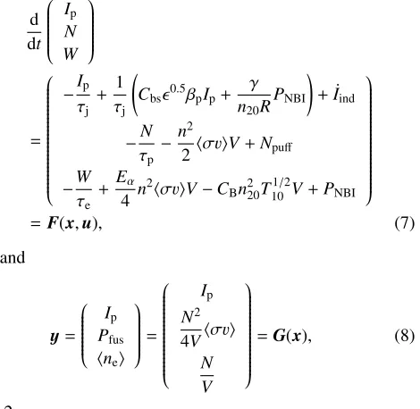
NBI, gas puffing, and induction current. As shown in the following equations, these control parameters are strongly coupled to the actuators. The state equation for the core plasma is described as follows:
d dt
⎛ ⎜⎜⎜⎜⎜ ⎜⎜⎜⎜⎝ INp
W ⎞ ⎟⎟⎟⎟⎟ ⎟⎟⎟⎟⎠ = ⎛ ⎜⎜⎜⎜⎜ ⎜⎜⎜⎜⎜ ⎜⎜⎜⎜⎜ ⎜⎜⎜⎜⎜ ⎜⎜⎜⎜⎜ ⎝
−Ip
τj +
1 τj
Cbs0.5βpIp+ γ
n20R
PNBI +I˙ind
−τN
p −
n2
2 σvV+Npuff −W
τe
+Eα
4 n
2σvV−C Bn220T
1/2
10 V+PNBI
⎞ ⎟⎟⎟⎟⎟ ⎟⎟⎟⎟⎟ ⎟⎟⎟⎟⎟ ⎟⎟⎟⎟⎟ ⎟⎟⎟⎟⎟ ⎠
=F(x,u), (7)
and
y=
⎛ ⎜⎜⎜⎜⎜ ⎜⎜⎜⎜⎝ PIfusp
ne ⎞ ⎟⎟⎟⎟⎟ ⎟⎟⎟⎟⎠= ⎛ ⎜⎜⎜⎜⎜ ⎜⎜⎜⎜⎜ ⎜⎜⎜⎜⎜ ⎜⎜⎜⎜⎝ Ip N2
4Vσv N V ⎞ ⎟⎟⎟⎟⎟ ⎟⎟⎟⎟⎟ ⎟⎟⎟⎟⎟
x=
⎛ ⎜⎜⎜⎜⎜ ⎜⎜⎜⎜⎝ INp
W ⎞ ⎟⎟⎟⎟⎟
⎟⎟⎟⎟⎠, (9)
u= ⎛ ⎜⎜⎜⎜⎜ ⎜⎜⎜⎜⎝ ˙ Iind PNBI
Npuff
⎞ ⎟⎟⎟⎟⎟
⎟⎟⎟⎟⎠, (10)
whereNis the total number of particles andW is the total stored energy. Values for the parameters are as follows [9]: γ=0.25, Cbs=0.782, Cb=0.032, (11)
τp=1 s, τj=100 s, (12)
βp=0.7, BT=5.3 T, (13)
R=6.2 m, a=2.0 m, κ=1.7, (14)
V =830 m3, Ai=2.5, (15)
τe=HH
×0.0562A0.19 i R
1.39
p a0.58κ0.78B0T.15I 0.93 P n
0.41 19 P−
0.69 tot .
(16) Since this state equation is nonlinear, linearization around the equilibrium point is performed. In this case, the target value is chosen as the equilibrium value of vec-torx, and from Eq. (7), the equilibrium value of vectoru
can be determined. The linearized state equation can be summarized as follows:
d
dtΔx=AΔx+BΔu, (17)
Δy=CΔx. (18)
The symbolΔindicates the deviation from the equilib-rium point for each parameter. We set the reference point to the equilibrium pointyref =yeqand require the controller to satisfy the equation as follows:
d
dtΔy=−K(y−yref)=−KΔy, (19)
K=
⎛ ⎜⎜⎜⎜⎜
⎜⎜⎜⎜⎝ 0.010 01 00
0 0 1
⎞ ⎟⎟⎟⎟⎟
⎟⎟⎟⎟⎠. (20)
The unit ofKis an inverce second (s−1), and diagonal
elements are determined from the inverse of the character-istic time for each state variable. In this situation, each component of the vectorΔyis expected to be dampened by its characteristic time. Thus, to get a suitable controller, we change the equations as follows:
d dty=
d dtΔy=C
d dtΔx=C
d
dtx, (21)
thus, d
dty=C AΔx+CBΔu, (22)
and d
dty=C AC
−1Δy+
CBΔu. (23)
From Eq. (19), we can obtain the actuator value as follows:
Δu=−(CB)−1K+C AC−1(y−y
ref). (24)
This is just a proportional controller. A proportional (P) controller, without the integral (I) and differential (D) controllers, cannot inhibit a disturbance or the effects of model errors. Thus, the I and D controllers should be added. On doing so, the controller is given as follows:
Δu=(CB)−1K+C AC−1(y−yref) −(CB)−1K2
t
0
(y−yref)dτ −(CB)−1K
3
d
dt(y−yref), (25) where
K2=
⎛ ⎜⎜⎜⎜⎜
⎜⎜⎜⎜⎝ 0.0010 0.10 00
0 0 0.1
⎞ ⎟⎟⎟⎟⎟
⎟⎟⎟⎟⎠, (26)
K3=
⎛ ⎜⎜⎜⎜⎜
⎜⎜⎜⎜⎝ 1.5×10
−4 0 0
0 0.015 0
0 0 0.015
⎞ ⎟⎟⎟⎟⎟
⎟⎟⎟⎟⎠. (27) The components inK2andK3are determined to make
the I and D terms comparable with the P term. Finally, a detailed adjustment is performed by trial and error. In gen-eral, if we perform PID control for three control parameters with three actuators, we need a 3×3 matrix for each P, I and D gain, i.e., (3×3)×3=27 components must be deter-mined. However, by introducing the state equation model, PID gains involving only diagonal matrices could be avail-able, requiring the determination of only 3×3 = 9 com-ponents. In addition, the characteristic time of each state equation variable is practical for determining PID gains.
4. MIMO Simulation for Core Plasma
For this MIMO system with a point model for core plasma, a feedback simulation was performed with the software Matlab/Simulink, which is an excellent tool for control simulation and controller design. Here (7) is solved by Matlab/simulink and actuators are evaluated from (25). Typical results for the time evolutions of the control pa-rameters and actuator values are shown in Figs. 3 and 4, respectively, where the reference values were set as fol-lows:y=
⎛ ⎜⎜⎜⎜⎜ ⎜⎜⎜⎜⎝ PIfusp
ne ⎞ ⎟⎟⎟⎟⎟ ⎟⎟⎟⎟⎠= ⎛ ⎜⎜⎜⎜⎜
⎜⎜⎜⎜⎝ 400 MW15 MA 1.0×10²⁰/m3
⎞ ⎟⎟⎟⎟⎟
⎟⎟⎟⎟⎠. (28) The initial control parameters are as follows:
x=
⎛ ⎜⎜⎜⎜⎜ ⎜⎜⎜⎜⎝ INp
W ⎞ ⎟⎟⎟⎟⎟ ⎟⎟⎟⎟⎠= ⎛ ⎜⎜⎜⎜⎜
⎜⎜⎜⎜⎝ 8.315 MA×1023
300 MW ⎞ ⎟⎟⎟⎟⎟
Fig. 3 Simulation results for time evolution of plasma currentIp, fusion powerPfusand plasma electron densityne.Ipand
neare maintained at their target values, while beginning at 250 s,Pfusfollows its target value from 400 to 500 MW and recovers from the disturbance at 300 s.
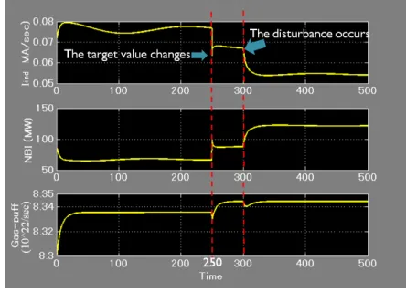
Fig. 4 Simulation results for the time evolution of the induced current ˙Ics, NBI power and amount of gas puff. At 250 s and 300 s, NBI power changes to drive the fusion power to its target. Simultaneously, the other two actuators change to keepIpandneconstant.
In Fig. 3, during the periodt = 0 - 250 s, control pa-rameters were maintained at target values with no offset. The controller was designed from the linearized form of the state equation given in (6).
At t = 250 s, the target value for fusion power was changed from 400 to 500 MW, while keeping values of the other two control parameters constant. In this case, the fusion power smoothly changed to the target value within 30 s with no offset. Simultaneously, the plasma current and plasma density remained constant. At this time, Figure 4 shows that the NBI power increased fromPNBI = 66 to
87 MW, so as to change the fusion power. Simultaneously, the induced current and the gas puff amount changed to keep the plasma current and plasma density at their refer-ence values.
Next, att =300 s, a deterioration in plasma confine-ment was simulated by changing the confineconfine-ment enhance-ment factor HH from 1 to 0.95, thereby simulating a distur-bance in plasma performance. Although the fusion power decreased slightly, it recovered within 40 s, and the devia-tion in fusion power was approximately 10%. Simultane-ously, NBI was increased to recover fusion power, while the induced current and gas puffamount were decreased to keep plasma current and plasma density constant.
5. Discussion and Summary
In this research, we performed a MIMO simulation for a fusion reactor in which three control parameters (i.e., fusion power, plasma current, and plasma density) were se-lected, and three actuators (i.e., NBI, gas puff, and induced current) were employed. By introducing an state equation on a point model for a core plasma, actuator values were smoothly determined. In addition, since the number of PID gains was significantly reduced, values for PID gains could be determined by a simple procedure.
In this simulation, the controller was designed within the framework of a physical model for a tokamak reactor, but the method is also suitable for helical or other types of fusion reactors. A similar 0D helical control simulation was reported in [10]. While in [11,12], a plasma parameter profile control experiment was reported in which parame-ter profile information was factored into well-known func-tions, and the controller was designed using a state equa-tion. However, in those studies, many diagnostics were used, and it might prove difficult to use the same methods in a future reactor. For this reason, in the future reactor, a plasma simulator will be necessary for profile control in which a plasma simulator would be expected to serve as an alternative to diagnostics.
In this research, the effects of model error (i.e. the er-ror between the model and the real system) were ignored. However, in a real reactor, the effects of model error will be critical. A control system that decreases the effects of model error will be required in the real reactor. For this problem, so-called robust control should be introduced into fusion reactor control. In Ref. [13], an H2 control simu-lation was performed with a 0D state equation and Mat-lab/Simulink; H2 control theory is one such robust control theory. In H2 control theory, the effects of model error are evaluated as the H2 norm, and the controller is designed to minimize the H2 norm. More recently, a more advanced infinity control theory has been developed. In the H-infinity theory, the effects of model error are evaluated as the H-infinity norm. To operate the future reactor, a robust control theory will be necessary. Therefore, an H-infinity control simulation with the 0-D time evaluate equation will be part of our future work.
Acknowledgement
Fujimoto who has advised me about the modern control theory. In addition, I appreciate Professor S. Matsuda who has made a discussion about the future reactor con-trol. Finally, the authors would like to thank Enago (www.enago.jp) for the English language review.
[1] J.A. Snapeset al., Fusion Eng. Des.85, 461 (2010). [2] B. Goncalves et al., Energy Convers. Manag. 51, 1751
(2010).
[3] Y. Kamada, J. Plasma Fusion Res. 86, 519 (2010) (in Japanese).
[4] A.E. Costley, IEEE Transaction on Plasma Science 38,
No10, OCTOBER (2010).
[5] K.M. Young, Fusion Sci. Technol.57, 298 (2010). [6] T. Suzuki, J. Plasma Fusion Res. 86, 530 (2010) (in
Japanese).
[7] Y. Miyoshiet al., Plasma Fusion Res.7, 2405135 (2012). [8] Graham C. Goodwinet al.,Control System Design
(Pren-tice Hall, 2000).