*Corresponding author’s e-mail: [email protected]
Harmony Search Algorithm for Location-Routing
Problem in Supply Chain Network Design
F. Misni2,3 and L.S. Lee1,2∗
1Laboratory of Computational Statistics and Operations Research, Institute for Mathematical Research, Universiti Putra
Malaysia, 43400 UPM Serdang, Selangor, Malaysia
2Department of Mathematics, Faculty of Science, Universiti Putra Malaysia, 43400 UPM Serdang, Selangor, Malaysia 3Centre for Mathematical Sciences, College of Computing and Applied Sciences, Universiti Malaysia Pahang, 26300,
Gambang, Pahang, Malaysia
The interdependence of facility location and vehicle routing has been recognized among the practitioners and researchers. The integration of these problems is more challenging in a supply chain network design problem. This paper considers a location-routing problem, which integrates the facility location problem and the vehicle routing problem. To effectively solved the problem, it is decomposed into three sub problems which are: location-allocation problem, multi-depot vehicle routing problem and multi-depot routing-allocation problem. The objective is to minimize the total operating facilities cost and the total travel distance cost between the depots and customers. A harmony search algorithm is proposed with several local optimisation approaches to further enhance the solution quality. The problem is tested with several benchmark dataset fr om the literature. The performance of the proposed algorithm is compared with other heuristic and metaheuristic approaches from the literature.
Keywords: harmony search; location-allocation; vehicle routing; supply chain
I. INTRODUCTION
The integration of short and long term decision planning in supply chain network design (SCND) has becomes the primary objective of many industries and companies. Along the process in SCND, decision making and coordination become the main issues (Rahmandoust & Soltani, 2019). The critical issues in supply chain are dealing with the routing of vehicle delivery, the strategic location of facilities and the allocation of the customers. Traditionally, the facility location and vehicle routing have been solved separately due to their complexity. However, these problems are connected to each other and the interdependencies of them will affect the optimal cost in the whole system of the supply chain. Location-routing problem (LRP) involved three main decisions: where to locate the strategic open depots, how to allocate the customers to the open depots, and how to minimize the distance route of vehicle to serve customers (Perl & Daskin, 1985). This problem is difficult to solve by the exact method especially for bigger data
set of depots and customers. Since the LRP is a NP-hard problem, the heuristic and metaheuristic methods are the preferred methods.
The warehouse location-routing problem (WLRP) was first solved by Perl and Daskin (1985). The authors used heuristic method and decomposed the problem into three sub problems; multi-depot vehicle routing problem (MDVRP), warehouse location-allocation problem (WLAP) and multi-depot routing allocation problem (MDRAP). Then, Hansen et al. (1994) modified the WLRP and solved with heuristic method improvised from Perl and Daskin (1985). Wu et al. (2002) considered the multi-depot location routing problem. They divided the problem into two phases, location-allocation at the first phase and a general vehicle routing problem at the second phase. The problem is solved in a sequential and iterative manner by simulated annealing.
49 decomposed into location-allocation and vehicle routing problem. A tabu search is used for the location phase to determine a good configuration of facilities to be used in the distribution. For the routing phase, an ant colony algorithm is run on the routing variable in order to obtain a good routing for the given configuration. The capacitated LRP problem was solved by Marinakis and Marinaki (2008) with a hybrid particle swarm optimization (HybPSO-LRP) that combines a PSO with the multiple phase neighbourhood search-greedy randomized adaptive search procedure (MPNS-GRASP) algorithm, the expending neighbourhood search (ENS) strategy and a path relinking (PR) strategy.
A new exact method based on a set-partitioning-like formulation of the problem is used to solve a capacitated LRP (Baldacci et al., 2011). The authors decomposed the lower bound in LRP produced by bounding procedures based on the dynamic programming and dual ascent methods into a limited set of multi capacitated depot vehicle routing problem. The same capacitated LRP is discussed under disruption (Zhang et al., 2015). The problem is solved by a metaheuristic based on maximum-likelihood sampling method, route-allocation improvement, two stage neighbourhood search and a simulated annealing. Göçmen and Erol (2018) constructed the two stages mathematical model to solve the LRP due to the complexity and computational time constraint.
In this paper, we proposed a Harmony Search (HS) algorithm to solve LRP in SCND since there is no research done in this domain. The value of harmony memory considering rate (HMCR) and pitch adjusting rate (PAR) is set to be dynamically changed during the execution. Multiple local neighborhood search and a generated population for the new solutions are also be implemented during the process of improvisation. The details of the LRP with the mathematical model and solution methods are explained in Section II. The proposed HS for LRP is presented in Section III. The algorithm is tested on several benchmark dataset of LRP and the results are analyzed in Section IV. The last section gives the conclusions of the study.
II. LOCATION-ROUTING
PROBLEM
LRP is a problem of solving the location of depots and the routing of vehicles. LRP is defined as determining the number and location of open depots, the allocation of customers to the depot and the delivery route of vehicle between the open depots and the assigned customers. Each of the established depots will
be imposed to the charges of fixed operating cost and the delivery is carried out once the depot is established. The cost of delivery is based on the total travel distance by the vehicles from the depot to the assigned customers.
In this paper, the objective of the LRP is to minimize the total fixed operating cost of the facilities and the total cost of traveled distance by the vehicles between the open depots and customers. The location of possible depots and customers are given and the demands of each customers to be served by vehicles are predetermined. The maximum capacity limit for depots and vehicles are also available.
A. Mathematical Modeling
The mathematical modeling of LRP is described as follows:
Set:
𝐼 = sets of all depots (𝑖 = 1,2, ⋯ , 𝐼)
𝐽 = sets of all customers (𝑗 = 1,2, ⋯ , 𝐽)
𝐾 = sets of all vehicles (𝑘 = 1,2, ⋯ , 𝐾)
Input parameter:
𝐷𝑗= demand of customer 𝑗
𝑑𝑖𝑗= distance from 𝑖 to 𝑗
𝑉𝑘= capacity of vehicle 𝑘
𝑁 = number of customer
𝐹𝑖= fixed operating cost of depot 𝑖
𝐷𝐶 = distance cost per miles
𝑉𝑖= maximum throughput at depot 𝑖
Decision variables:
𝑈𝑙𝑘= auxiliary variable for sub-tour elimination constraints in vehicle 𝑘 of customer 𝑙
𝑧𝑖= {1, if depot 𝑖 is open0, otherwise
𝑦𝑖𝑗= {1, if depot 𝑖 assign to customer 𝑗0, otherwise
𝑥𝑖𝑗𝑘= {1, if arc (𝑖, 𝑗) is travelled by vehicle 𝑘0, otherwise
min 𝑓 = ∑ 𝐹𝑖 𝑖∈𝐼
𝑧𝑖+ ∑ ∑ ∑ 𝐷𝐶 × 𝑑𝑖𝑗𝑥𝑖𝑗𝑘 𝑘∈𝐾
𝑗∈𝐼∪𝐽 𝑖∈𝐼∪𝐽
(1)
50
∑ ∑ 𝑥𝑖𝑗𝑘
𝑖∈𝐼∪𝐽 𝑘∈𝐾
= 1 , ∀𝑗 ∈ 𝐽 (2)
∑ ∑ 𝑥𝑖𝑗𝑘 𝑗∈𝐽 𝑖∈𝐼 ≤ 1 , ∀𝑘 ∈ 𝐾 (3)
∑ ∑ 𝐷𝑗𝑥𝑖𝑗𝑘 𝑗∈𝐽 𝑖∈𝐼∪𝐽 ≤ 𝑉𝑘 , ∀𝑘 ∈ 𝐾 (4)
∑ 𝑥𝑖𝑗𝑘 𝑖∈𝐼∪𝐽 − ∑ 𝑥𝑖𝑗𝑘 𝑗∈𝐼∪𝐽 = 0 , ∀𝑖 ∈ 𝐼 , ∀𝑘 ∈ 𝐾 (5)
∑ 𝐷𝑗𝑦𝑖𝑗 𝑗∈𝐽 ≤ 𝑉𝑖𝑧𝑖 , ∀𝑖 ∈ 𝐼 (6)
𝑈𝑙𝑘− 𝑈𝑗𝑘+ 𝑁𝑥𝑙𝑗𝑘≤ 𝑁 − 1 , ∀𝑙, 𝑗 ∈ 𝐽, ∀𝑘 ∈ 𝐾 (7)
∑ 𝑥𝑖𝑢𝑘+ 𝑥𝑢𝑗𝑘− 𝑦𝑖𝑗≤ 1 , ∀𝑖 ∈ 𝐼 , ∀𝑗 ∈ 𝐽 , ∀ 𝑢∈𝐼∪𝐽 𝑘 ∈ 𝐾 (8)
𝑦𝑖𝑗∈ {0,1} , ∀𝑖 ∈ 𝐼 , ∀ 𝑗 ∈ 𝐽 (9)
𝑥𝑖𝑗𝑘∈ {0,1} , ∀𝑖 ∈ 𝐼 ∪ 𝐽 , ∀𝑗 ∈ 𝐼 ∪ 𝐽 , ∀𝑘 ∈ 𝐾 (10)
𝑧𝑖∈ {0,1} , ∀𝑖 ∈ 𝐼 (11)
𝑈𝑙𝑘≥ 0 , ∀𝑙 ∈ 𝐽 , ∀𝑘 ∈ 𝐾 (12)
The objective of LRP in Eqn.(1) is to minimize the total fixed operating cost of depots and the total distance cost traveled by the vehicles. Constraints in Eqn.(2) and (3) indicate that, each of the customers has to be assigned in a single route and it can be served by only one vehicle. The total demands at each route cannot exceed the vehicle capacity limit and the vehicle must start and end at the same depot. These two constraints are shown in Eqn.(4) and (5), respectively. Besides vehicle capacity limit, the capacity constraint for depot is given in Eqn.(6). Eqn.(7) represents the new sub tour elimination constraint and Eqn.(8) specified that the customer will be assigned to the depot if there is a route from that depot. The binary values on decision variable and the positive values for auxiliary variable are defined in Eqn.(9) - (12), respectively.
In order to solve the LRP problem, the problem is divided into three sub problems and solved sequentially, which are: location-allocation problem, multi-depot vehicle routing problem, and multi-depot routing-allocation problem.
1. Location-allocation Problem
In the location-allocation problem, each of the customers is initially assigned to the nearest depots based on the Euclidean distance formulation. The customers will be moved around to the possible depots during the process of improvisation. The
vehicle capacity limit constraint has been relaxed in order to minimize the number of open depots and assumed only one vehicle is being used at each depot. However, the depot capacity limit should not be violated during the process.
2. Multi-depot Vehicle Routing Problem
After the number and location of open depots are determined, the allocation of customers at each depot need to be sequenced and divided into vehicles according to the vehicle capacity limit. This process is performed among the open depots only. The process of local optimisation is focusing within the open depots. Both depot capacity limit and vehicle capacity limit should not be violated.
3. Multi-depot Routing-allocation Problem
The last subproblem is to reallocate the customers to the possible closed depots and solved the routing problem. To identify the possible closed depot to be opened is based on the stem distance. Stem distance is the distance between the depot to the first customers and between the last customers to the depot of each route. The customer’s route will be moved to another closed depot if the stem distance is reduced as compared to the current depot. The local optimisation is applied during the vehicle route improvisation process.
B. Proposed Harmony Search Algorithm
Harmony Search (HS) is a popular-based metaheuristic algorithm that imitates the music improvisation of a group orchestra (Geem et al., 2001). The musician will improvise their harmony with these three options:
i) select any pitch that has been played from the previous harmony memory,
ii) fix the pitch that sound similar to any previous pitch in the memory , or
51 metaheuristic methods that shown the promising performance when solving the NP-hard optimization problem (Askarzadeh & Rashedi, 2018). In this paper, the modifications that have been implemented in the proposed HS algorithm are detailed below.
Step 1: Initialization
In HS, several solutions are generated to produce an initial population. The solutions can be generated either randomly or by a heuristic. In the proposed HS, a random initial population called harmony memory (HM) is created and sorted according to their fitness values. The number of solutions in the HM is the harmony memory size (HMS). HM can be described in the following matrix:
= ) ( ) 2 ( ) 1 ( 2 1 2 2 2 1 2 1 2 1 1 1 xHMS f x f x fxHMSn xn xn xHMS x x xHMS x x HM (13) where,
𝑥𝑖𝑗= decision variable for 𝑖 = 1,2, ⋯ , 𝑛 and 𝑗 = 1,2, ⋯ , 𝑀𝐻𝑆 ,
𝑓(𝑥𝑗) = fitness function of 𝑥𝑗 for 𝑗 = 1,2, ⋯ , 𝑀𝐻𝑆 .
Step 2: Parameter Setting
The parameters setting used in the proposed HS algorithm are HMCR, PAR, HMS and the stopping criterion. An appropriate value of HMCR will lead to the choices of good solutions as element of new solutions. The solution may not well explored if the value of HMCR is too high. But if it is too low, only few good solutions are selected for next iteration. Same goes to PAR, a higher value of PAR is not recommended as it can cause the solutions to be stucked at the local optima. The convergence speed may be slow if the value of PAR is too small. Therefore, in order to use the memory effectively, the value of HMCR should be in between 0.7 and 0.95 and the value of PAR is supposed to be in between 0.1 and 0.5 (Yang, 2009). However, this range may be suitable and valid for some problems only.
Instead of using a fixed value, the proposed HS used a dynamic value of HMCR and PAR by using the following formulation in order to balance the exploration and exploitation:
𝐻𝑀𝐶𝑅𝑖𝑡= 𝐻𝑀𝐶𝑅𝑚𝑎𝑥− (𝐻𝑀𝐶𝑅𝑚𝑎𝑥− 𝐻𝑀𝐶𝑅𝑚𝑖𝑛) 𝑖𝑡
𝑀𝑎𝑥𝐼𝑡 , (14)
𝑃𝐴𝑅𝑖𝑡= 𝑃𝐴𝑅𝑚𝑎𝑥− (𝑃𝐴𝑅𝑚𝑎𝑥− 𝑃𝐴𝑅𝑚𝑖𝑛)𝑀𝑎𝑥𝐼𝑡𝑖𝑡 , (15) where,
𝑖𝑡 = the current iteration,
𝑀𝑎𝑥𝐼𝑡 = the maximum iterations,
𝐻𝑀𝐶𝑅𝑚𝑎𝑥= the maximum value of the HMCR,
𝐻𝑀𝐶𝑅𝑚𝑖𝑛= the minimum value of the HMCR,
𝑃𝐴𝑅𝑚𝑎𝑥= the maximum value of the PAR,
𝑃𝐴𝑅𝑚𝑖𝑛= the minimum value of the PAR.
This formulation is introduced by Mahdavi et al., (2007), but with a slight modification. The proposed HMCR and PAR are reduced gradually when there is no improvement found in the solution. In this problem, the range values of HMCR and PAR are set to be [0.7,0.95] and [0.3,0.9] respectively. The reason of reducing the HMCR slowly is to increase the probability of exploring more solution space not in the HM. Hence, the global optimal can be attained (Alia & Mandava, 2011). The dynamic value of HMCR and PAR can avoid the solutions getting trapped in the local optimum quickly.
Step 3 : Improvisation
Generate the new solution
A standard HS (SHS) utilize a single search solution to evolve. This makes the algorithm converged slowly to the optimal solution. To increase the speed of convergence, several new solutions are generated at each iteration and called as HMnew in the proposed HS. The size of HMnew is smaller than the size of HM. A new solution is taken from the HM randomly with the probability of HMCR, otherwise it will be generated randomly within the range of the harmony vector. The SHS assumed that each solution in the HM has the same probability to be chosen as a new solution (Zhang & Geem, 2019). However in the proposed HS, HM will be divided into two sub population equally which are HMbest and HMworst according to the ranking of the fitness values. The first rank in HM is the best solution and the last rank will be the worst one. The best HM will be used to explore and exploit the solution while the worst HM is used to explore the solution only.
Local neighborhood search
52 HS implements the multi local neighborhood search. The techniques of local search are divided into two: within a depot and between two depots. Four techniques of neighborhood search are used which are swap (either swapping within depot or between depots), insertion and relocation. The local search is applied to the new solution with the probability of PAR. At each iteration, the process of generating new solution and local search are repeated until the number of harmony vectors equal to the size of HMnew.
Swap: exchange the position of two random customers within the same route or between different routes. Swapping can be done within a same depot or between the depots.
Insertion: insert a customer in between two other random customers within a same depot.
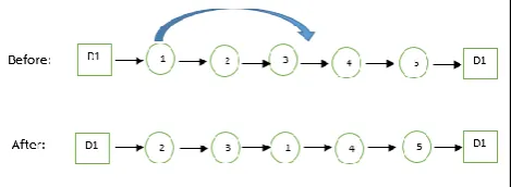
Relocation: relocate the customers from the current depot to a new depot.
Swapping within a depot and insertion are two techniques that involve the searching of the neighborhood within a same depot while swapping between two depots and relocation are techniques that require two different depots. In location-allocation phase and multi-depot vehicle routing phase, the closed depots will not be considered during the local search process. The example of these techniques are graphically shown in Figure 1-4.
Figure 1. Swapping two customers within the same depot
Figure 2. Inserting a customer in between two customers
Figure 3. Swapping two customers between two depots
Figure 4. Relocating a customer of depot 2 to depot 1
Step 4: Update HM
To update the solutions in HM, the HMnew created at each iteration is combined together with current HM. The solutions are sorted according to the value of objective function. The best solution with the size of HMS will be kept for the next iteration.
Step 5: Stopping criteria
The proposed algorithm will be terminated when 100 consecutive non-improving iteration are performed.
53
III. RESULTS AND DISCUSSION
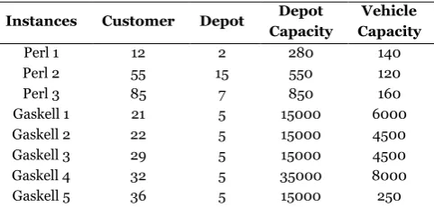
The proposed HS is implemented in MATLAB software R2017b and tested with benchmark dataset of Perl and Gaskell. The characteristics of the dataset are given in Table 1.
Table 1. Perl and Gaskell dataset
Instances Customer Depot Depot
Capacity
Vehicle Capacity
Perl 1 12 2 280 140
Perl 2 55 15 550 120
Perl 3 85 7 850 160
Gaskell 1 21 5 15000 6000
Gaskell 2 22 5 15000 4500
Gaskell 3 29 5 15000 4500
Gaskell 4 32 5 35000 8000
Gaskell 5 36 5 15000 250
For Perl dataset, the proposed HS is compared with other literature that used heuristic method (Heuristic) (Perl & Daskin, 1985), simulated annealing in Wu et al. (2002) (SA-W) and in Zhang et al. (2015) (SA-Z), hybrid tabu search and ant colony (Tabu-ACO) (Wang et al., 2005) and particle swarm optimisation (PSO) (Marinakis & Marinaki, 2008). For Gaskell dataset, the proposed HS is compared with different variants of particle swarm which are particle swarm optimisation (PSO), PSO with MPNS-GRASP (PSO-MPNS-GRASP), PSO with MPNS-GRASP and ENS (PSO-MPNS-GRASP-ENS) and hybrid
PSO (HybPSO-LRP) in Marinakis and Marinaki (2008) and the honey bee mating optimization (HBMO) in Marinakis et al. (2008) as well. The results of these comparison are presented in Table 2 and Table 3. A SHS is also included for both experiments.
Table 2. Comparative results of Perl dataset
Method Perl 1 Perl 2 Perl 3
Heuristic 203.97 1146.13 1657.60
SA-W 203.97 1119.83 1656.72
Tabu-ACO 203.97 1139.87 1642.57 PSO 203.97 1135.90 1656.90
SA-Z 203.97 1115.40 1642.00
SHS 203.97 1158.80 1832.10 Proposed HS 203.97 1113.24 1652.99
Table 3. Comparative results of Gaskell dataset Methods Gaskell 1 Gaskell 2 Gaskell 3 Gaskell 4 Gaskell 5
PSO 437.1 592.1 512.1 574.1 470.7
PSO-MPNS-GRASP
435.9 591.8 512.1 571.7 470.7
PSO-MPNS-GRASP-ENS
435.9 591.7 512.1 571.7 470.7
HybPSO-LRP 432.9 588.5 512.1 570.8 470.7 HBMO 431.9 587.2 512.1 569.8 470.7 SHS 443.7 598.0 541.2 576.2 520.7 Proposed HS 431.7 577.0 511.8 559.9 464.1
54 Figure 5. 12 customers and 2 depots
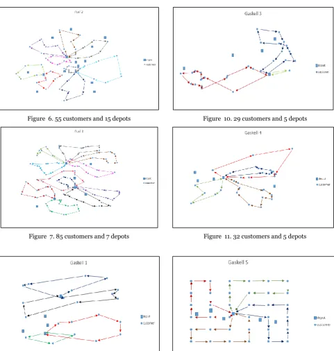
Figure 6. 55 customers and 15 depots
Figure 7. 85 customers and 7 depots
Figure 8. 21 customers and 5 depots
Figure 9. 22 customers and 5 depots
Figure 10. 29 customers and 5 depots
Figure 11. 32 customers and 5 depots
55
IV. CONCLUSIONS
In this paper, a modified HS is proposed for solving the LRP which is divided into three subproblems: location-allocation problem, multi-depot vehicle routing problem and multi-depot routing-allocation problem. In the SHS, the new solution is generated once at each iteration with a fixed value of HMCR and PAR. Meanwhile in the proposed HS, the multi solutions are generated and multi neighborhood search techniques are implemented during the process of improvisation based on the value of PAR. Both HMCR and PAR are changed dynamically when there is no improvement found in the solution. In order to increase the intensification capability, the HM is divided into two subpopulation called HMbest and HMworst. Two
well-known benchmark dataset of Perl and Gaskell are used to evaluate the proposed algorithm. The results shown that the proposed HS is efficient to be implemented in LRP and successful in obtaining better solutions for most instances.
V. ACKNOWLEDGEMENT
This research was supported by the Geran Putra-Inisiatif Putra Siswazah (GP-IPS/2017/9579400), Universiti Putra Malaysia (UPM). The authors would like to thank reviewers for their time to thoroughly review and provide constructive comments for improvements of the manuscript.
VI. REFEREENCES
Alia, OM & Mandava, R 2011, ‘The variants of the harmony search algorithm: an overview’,Artificial Intelligence Review, vol. 36, no. 1, pp. 49-68.
Askarzadeh, A & Rashedi, E 2018, Harmony search algorithm: basic concepts and engineering applications. In intelligent
systems: concepts, methodologies, tools, and applications, IGI Global, pp. 1-30.
Baldacci, R, Mingozzi, A & Wolfler Calvo, R 2011, ‘An exact method for the capacitated location-routing problem’, Operations Research, vol. 59, no. 5, pp. 1284-1296.
Geem, ZW, Kim, JH & Loganathan, GV 2001, ‘A new heuristic optimization algorithm: harmony search’, Simulation, vol. 76, no. 2, pp. 60-68.
Göçmen, E & Erol, R 2018, ‘Location and multi-compartment capacitated vehicle routing problem for blood banking system’,International Journal of Engineering Technologies, vol. 4, no. 1, pp. 1-12.
Hansen, PH, Hegedahl, B, Hjortkjaer, S & Obel, B 1994, ‘A heuristic solution to the warehouse location-routing problem’, European Journal of Operational Research, vol. 76, no. 1, pp. 111-127.
Mahdavi, M, Fesanghary, M & Damangir, E 2007, ‘An improved harmony search algorithm for solving optimization problems’,Applied Mathematics and Computation, vol. 188, no. 2, pp. 1567-1579.
Marinakis, Y & Marinaki, M 2008, ‘A particle swarm optimization algorithm with path relinking for the location routing problem’, Journal of Mathematical Modelling and Algorithms, vol. 7, no. 1, pp. 59-78. Marinakis, Y, Marinaki, M & Matsatsinis, N 2008, ‘Honey
bees mating optimization for the location routing problem’,IEEE International Engineering Management Conference, pp. 1-5.
Perl, J & Daskin, MS 1985, ‘A warehouse location-routing problem’, Transportation Research Part B: Methodological, vol. 19, no. 5, pp. 381-396.
Rahmandoust, A & Soltani, R 2019, ‘Designing a location-routing model for cross docking in green supply chain’, Uncertain Supply Chain Management, vol. 7, no. 1, pp. 1-16.
Wang, X, Sun, X & Fang, Y 2005, ‘A two-phase hybrid heuristic search approach to the location-routing problem’, IEEE International Conference on Systems, Man and Cybernetics, vol. 4, pp. 3338-3343.
Wu, TH, Low, C & Bai, JW 2002, ‘Heuristic solutions to multi-depot location-routing problems’, Computers & Operations Research, vol. 29, no. 10, pp. 1393-1415. Yang, XS 2009, Harmony search as a metaheuristic
56 Zhang, T & Geem, ZW 2019, ‘Review of harmony search with
respect to algorithm structure’, Swarm and Evolutionary Computation, vol. 48, pp. 31-43.