Continuous Free-Electron State-Density Modeling
Based on Plasma Microfield
Takeshi NISHIKAWA
Graduate School of Natural Science and Technology, Okayama University, 3-1-1 Tsushima-naka, Okayama 700-8530, Japan
(Received 19 June 2012/Accepted 20 August 2012)
Following the atomic model based on the microfield in a plasma for bound states [Astrophysical Journal
532, 670 (2000)], I have considered an atomic modeling for computing the free-electron state-density based on the plasma microfield. In the atomic model based on the plasma microfield, it is considered that an ion in plasma is immersed in a uniform electric field that is the contribution of field values averaged over the other ions in the plasma. It has been expected a modeling for the free-state density consistent with its bound state, because the resulting free-state densities by the simple atomic model based on the plasma microfield has been found to be invalid. In this study, I have obtained a physically appropriate free-state density under the assumption that the large electric field component can be considered to exist due to the electric field originating from the nearest neighboring ion and the resulting potential around the ion shows mirror symmetry about the saddle point. The resulting state density is consistent with the experimental results. The inclusion of the free-state density has caused a slight deviation in the values of the average ionization degree of hydrogenic plasmas.
c
2012 The Japan Society of Plasma Science and Nuclear Fusion Research
Keywords: free state, statistical weight, state density, Saha-Boltzmann, microfield, average ionization degree DOI: 10.1585/pfr.7.1401142
1. Introduction
Final objective of this study is finding a method to compute the degree of ionization of plasma, which is es-sentially the analysis of the atomic processes occurring in plasma, based on the plasma microfield. First, I reexam-ine the conventional method to compute the degree of the ionization of plasmas and show the importance of the state density modeling to the resulting values of the average ion-ization degree.
In the state of local thermodynamic equilibrium (LTE), the ratio of the product of the number density of the (Z+1)-charged ionNZ+1, and that of the electron Ne(E) of its energy E, to that of the combined Z-charged ion
NZ, is determined by the ratio of the statistical weights of the states of the (Z +1)-charged ionUZ+1 to that of the
Z-charged ionUZ, the Boltzmann factor between the two states as given by exp(−(E+Ip)/kBTe), and the number of electron states in free space per unit volume 2(4πp2/h3)dp, i.e.,
NZ+1Ne(E)
NZ
= UZ+1
UZ exp
−E+Ip
kBTe
24πp 2
h3 dp. (1) In the expression involving the Boltzmann factor, Ip,kB, andTedenote the ionization potential from theZ-charged to the (Z+1)-charged state, the Boltzmann constant, and the electron temperature, respectively. In the expression involving the number of electron states,hdenotes Planck’s constant. With respect to the energy of the free electron
author’s e-mail: [email protected]
and its momentump, the expressionE = p2/2m
eis satis-fied, and here,medenotes the mass of the electron. Trans-lating the free electron’s momentum to its equivalent en-ergy and integrating Eq. (1) over the enen-ergy range of the free electron forE>0, we obtain
NZ+1Ne
NZ =
UZ+1
UZ exp
− Ip
kBTe
8π2me3
h3
×
∞
0
√ Eexp
− E
kBTe
dE = UZ+1
UZ exp
− Ip
kBTe
2
2πmekBTe
h2
3/2
.(2)
This equation is called the Saha-Boltzmann equation. Ap-plying the equation to various ionic species including their excited states in plasma, we can compute the population of all ionic species in the plasma along with the average ionization degree obtained byZav=Ne/N0from this com-puted population, whereN0is the total number density of ion and atom defined byNZ.
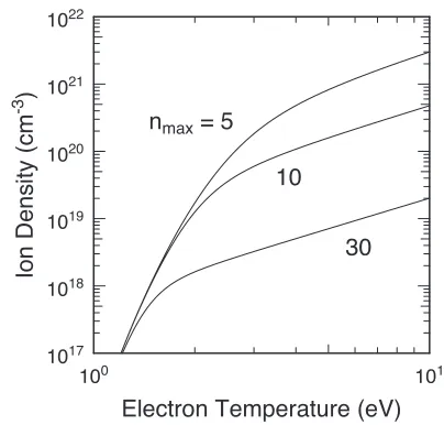
Practically, we need to determine the number of bound states when we apply the Saha-Boltzmann equation for re-alistic plasmas. For the case of hydrogenic plasmas, Fig. 1 shows one of the difficulties arising out of the convention-ally used simple model in which the bound states exist up to a fixed maximum principal quantum number. The con-tours for an average ionization degree of 0.5 are plotted for three cases in which the maximum principal quantum numbers of the considered bound states aren=5, 10, and
c
Fig. 1 Contours of average ionization degree are 0.5 of hydro-genic plasmas. The maximum principal quantum num-bers of the considered bound states aren = 5, 10, and 30.
30. From Fig. 1, it can be observed that the plasma den-sity and its temperature for an average ionization degree of 0.5 varies depending on the maximum principal quantum number of the bound state in the atomic process model. In other words, the plasma density and its temperature for an average ionization degree of 0.5 can be varied by changing the maximum principal quantum number.
In order to address this ambiguity, Nishikawa has suggested a simple analytical expression that allows for the counting of the number of bound states based on the plasma microfield [1]. In the model, hydrogenic ions are assumed to be immersed in a statistically distributed uni-form electric field, i.e., the microfield in the plasma. As a result, the potential profile around the ion in plasma is given by the superposition of the ion’s Coulomb potential
Zae/4π0r and the potential due to the uniform external fieldF; here, Za,e, and 0 denote the nuclear charge of the ion, the elementary charge, and the permittivity of free space, respectively. The hydrogenic ion has a bound state whose energy is given by−mee4Za2/802h2n2, and this en-ergy is assumed to be unchanging even in the external elec-tric field. In this case, the potential distribution around the ion shows a saddle point. The height of the saddle point varies as the function of the strength of the uniform exter-nal electric field. I determine that the electronic state is that of a free electron for energies above this saddle point and that the energy values below the saddle point indicate bound states. Although we now know this is to be quantum mechanically false, this picture can still provide a conve-nient basis for further improved treatment. From the above assumption, the threshold electric field till which the bound statenexists is given as
Fcn=
πme2e5Za3 6403h4n4
. (3)
Although a minor correction factor may be required in the equation, its contribution of determining the threshold principal quantum numbern from the electric field Fncis expected to be of the order of the one fourth power of the factor. The probability that the bound statenexists is given by the expression
wn=
Fc n
0
dF P(F), (4)
whereP(F) represents the distribution function of the mi-crofield. Using the Holtsmark field, given as
H(β)=F0W(F)= 2
πβ
∞
0
xexp[−x3/2] sin(βx) dx,
(5) as the statistically distributed uniform microfieldF, we can compute Eq. (4), whereβ=F/F0, as
F0=2π
4Np 15
2/3 Z pe 4π0,
(6)
whereNpandZpdenote the number density and the charge state of the perturbing ion, respectively. The termF0 is called the Holtsmark normal field strength [2]. The Holts-mark field is obtained by summing up the contribution of the electric field from evenly spread ions over space, i.e., the Coulomb interaction between two ions is neglected. Under certain circumstances where the kinetic energy of ions is considerably larger than that of the interaction, the field distribution given by the Holtsmark field becomes ap-propriate. The simple expression for the probability that the bound state exists, as derived in Ref. [1], is obtained by using the approximation thatH(β)∼4β2/3πnearβ=0. It must be noted that given by the equations used in Ref. [1] are incorrect. The correct expression for the probability of the statenis given by
wn=
Fc n
0
dFP(F)= 5 2Z
a9 217π4n12Z
p3Np2
, (7)
i.e., not the 8th power ofZabut the 9th power ofZa. For the hydrogenic case,Za=Zp=1.
2. State Density for Free Electron
based on Plasma Microfield
In the conventional atomic process modeling, the translation of the electron’s momentum to its equivalent energy in the free-state density calculations is carried out using the equationsE=p2/2m
eand 2·4πp2dp/h3. In the present modeling, an ion is assumed to be in a potential that is composed of the Coulomb potential of its nucleus and the potential due to the uniform external field. To ac-commodate this effect, we rewrite the relation between the electron’s energy and momentum at (r, θ) in the spherical coordinates inside the ion sphere radiusR0as
p2
2me =
E+ 1
4π0
Zae2
r +eFrcosθ. (8)
The ion sphere has a radiusR0such that 4π
3 R0 3N
i=1. (9)
The second term on the right hand side of Eq. (8) indicates the contribution of the Coulomb potential of the nucleus and the third term indicates that of the plasma microfield. This relation shows that even if the electron energy is zero, its momentum does not become zero, i.e., the electron has sufficient kinetic energy to overcome the attractive force of the nucleus from the classical point of view. The state density of the free electron including the potential effect is
f(E)=8π
2me3
h3
∞
0
H(β) dβ
R0
0
2πr2dr
×
π
0
sinθdθ
E+ 1
4π0
Ze2
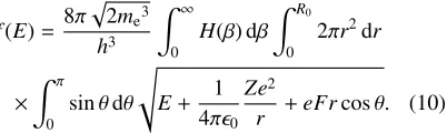
r +eFrcosθ. (10)
In the modeling, the free-state density is computed within the ion sphere of radius R0. Figure 2 shows the free state density of hydrogenic plasma with ion densityNi = 1016cm−3 for various values ofβmax. The term βmax in-dicates the maximum value of the integral range ofβ in Eq. (10). The reduced statistical weights of the bound states have been computed by using Eq. (4), and not by using Eq. (7). ForE0, the free state density defined by Eq. (10) asymptotically approaches 8π2me3E/h3. The energy is normalized by twice the hydrogenic ionization potential, 2ERy. To understand the continuity of the state densities, we show the bound states as a reduced contin-uous bound state with a statistical weight 2n2 spread over the energy range between the next higher state and the next lower state that leads to an area equal to its original sta-tistical weight 2n2/(E
n+1/2−En−1/2), i.e., the area below each step in Fig. 2 is equal to 2n2. The reduced continu-ous bound state profile converges to the the asymptotic be-havior of the number of bound state below E = 0 given by 2−3/2(−E)−5/2, as calculated by the relation given by Eq. (8) without including the third term. It may be noted that the vertical axis represents the logarithm scale. The
Fig. 2 State densities of free and bound states as obtained by simple atomic model based on plasma microfield for var-ious values ofβin Eq. (10). However, the state density of the free electron becomes larger than that of its bound state for the same energy although the values of the free-state density does not diverge.
numbers indicate the principal quantum numbers of the state. Hereafter, we refer to the reduced continuous bound state profile as the reduced bound state density. The two-dot chain curves show the asymptotic bound state density given by 2−3/2(−E)−5/2, and the state density of electron in free space, 82πme3E/h3, for reference.
From Fig. 2, we can see that the free state density does not become zero at E = 0, and it further exists below
E = 0. However, the free-state density obtained by the simple atomic model based on the microfield is not practi-cally acceptable since the free-state density has been com-puted as larger than that of a bound electron of the same energy although the values of the state density does not di-verge. The effect on the ion-ion correlation is small in the case of the small ion number density values discussed here. The value ofΓ, which is the ratio of the potential energy of two ions in the plasma to its temperature, is nearly equal to 0.05 when the temperature of the hydrogenic plasma with ion density Ni = 1016cm−3 is 1 eV. Detailed investiga-tions show that the difficulty is induced on the potential far beyond the saddle point inside the ion sphere of ra-diusR0. Such a large electric field by which the saddle point is sufficiently inside the ion sphere occurs even in the low density plasmas, although the probability is rel-atively small. The position of the saddle point is given by rs =
Zae/4π0βF0, while the ion sphere radius is given by Eq. (9). From the equations, it is observed that the saddle point exists within the ion sphere radius when
Fig. 3 Schematic figure illustrating potential modification to overcome difficulty arising in simple atomic model in-cluding plasma microfield when saddle point of potential is within ion spere radius.
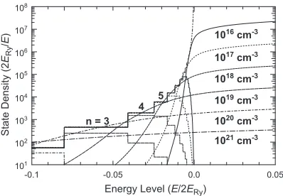
Fig. 4 State density with modification in potential assuming the mirror symmetry with respect to saddle point for vari-ous ion number densities ranging fromNi=1016cm−3to 1021cm−3for fully ionized hydrogenic plasmas.
symmetry of the potential with respect to the saddle point. Thus, the potential by which the free-state density is com-puted is indicated by the solid curve instead of the thick dashed curve in Fig. 3.
Figure 4 shows the energy dependence of the state densities of the free and bound states of hydrogenic plasma by using the above-mentioned potential modeling. The energy dependence curves are plotted for six cases from
Ni =1016cm−3 to 1021cm−3. From Fig. 4, we can under-stand that the difficulty in the previous computation is in-duced by the contribution of the potential on the free-state density from far beyond the saddle point, and the free-state densities do not exceed the corresponding asymptotic re-duced bound state densities for the same energy.
The quantum states up to the principal quantum num-ber of n = 8 are almost completely existing for Ni = 1016cm−3. From the state value ofn =9, the bound state densities gradually decrease, while the free-state density
Fig. 5 Average ionization degree of hydrogenic plasma. The po-tential is assumed to be mirror symmetry with respect to the saddle point.
appears and gradually increases as the principal quantum number becomes larger. Experimentally [3], the bound-bound spectrum from for state values n = 2 to 8 in hy-drogenic plasma withNi =1.8×1016cm−3can be clearly observed, while those for n ≥ 9 are merged with the free-bound spectrum although the bound-bound spectrum is broadened due to the Stark effect. For Ni = 9.3 × 1016cm−3 in Ref. [3], the bound-bound spectra from for state values ofn = 2 to 6 can be clearly observed while our model posits bound state existence up to n = 6 for
Ni = 1017cm−3. From our analysis, we might be able to provide a physical meaning for the pseudo-continuum that has been introduced by Däppen [4]. In this light, fu-ture studies would be required to examine the state density computation in which the potential distribution and profile of the nearest neighboring ion are actively considered.
Using the model, we can also compute the average ionization degree of various plasmas. In the case of the present model, the free state density f(E) is used instead of √Ein Eq. (2), i.e.,
NZ+1Ne
NZ =
UZ+1
UZ exp
− Ip
kBTe
×
∞
max(−e2Z
4π0r−eFrcosθ,−2e
eZ
aF 4π0)
f(E) exp
− E
kBTe
dE.
(11) It is noted that the lower range of the integration onEhas been changed to be from 0 to the larger value of just poten-tial at the point,−e2Z/4π
0r−eFrcosθor potential at the saddle point, −2e
eZaF
free-state density deviate slightly to the lower temperature region since the free-state density exists continuously from the bound state. The deviation is not very large; however, the deviation grows larger as the plasma density increases. In conclusion, I draw attention to one of the features of the present model in comparison with other models in which the concept of the ion sphere is used [5]. Most atomic models that apply the concept of an ion sphere only consider the plasma effects on the resulting potential in a spherical fashion. Therefore, we sometimes encounter the difficulty of the sudden disappearance of a bound state at a given threshold density when we compute the average ion-ization degrees over a wide range of plasma density and temperature. Using the present model, we can avoid such difficulties since the bound states gradually decrease as the density increases.
3. Summary
In this study, I have considered an atomic model to compute the free-electron state-density based on the mi-crofield in a plasma. In the atomic modeling based on the plasma microfield, it is considered that an ion in plasma is immersed in a uniform electric field that is the contribution of the field values averaged over the other ions in the plasma. The Holtsmark Field is used to obtain the distribu-tion of the uniform electric field in plasma throughout this study. However, the resulting free-state densities obtained by the simple atomic model are invalid, i.e., the free-state
density becomes larger than those of the bound states. The problem arises from the presence of a large electric field component, although its probability of occurrence is rela-tively small. A large free-state density is induced on the potential far beyond the saddle point inside the ion sphere radius. If the large electric field component can be consid-ered to exist due to the electric field originating from the nearest neighboring ion, and the resulting potential around the ion is assumed to show mirror symmetry with respect to the saddle point when the nearest neighboring ion is within the ion sphere, the physically appropriate free-state den-sity, which appears when the bound state disappears, can be computed. The resulting state density is consistent with the experimental results. The inclusion of this effect causes a slight deviation in the values of the average ionization de-gree of hydrogenic plasmas. This model is different from most other former models previously used since the state densities of the free and bound electron are computed us-ing a non-spherical potential profile.
[1] T. Nishikawa, Astrophysical J.532, 670 (2000).
[2] H.R. Griem,Spectral line broadening by plasmas(Academic Press, New York, 1974) p. 17.
[3] W.L. Wiese, D.E. Kelleher and D.R. Paquette, Phys. Rev. A
6, 1132 (1972).
[4] W. Däppen, L. Anderson and D. Mihalas, Astrophysical J.
319, 195 (1987).
[5] For example, I. Shimamura and T. Fujimoto, Phys. Rev. A