Spectral Interpolation on 3
×
3 Stencils for
Prediction and Compression
Lorenzo Ibarria
Georgia Institute of Technology, Atlanta, GA, USA Email:[email protected]
Peter Lindstrom
Lawrence Livermore National Laboratory, Livermore, CA, USA Email:[email protected]
Jarek Rossignac
Georgia Institute of Technology, Atlanta, GA, USA Email:[email protected]
Abstract— Many scientific, imaging, and geospatial applications produce large high-precision scalar fields sampled on a regular grid. Lossless compression of such data is commonly done using predictive coding, in which weighted combinations of previously coded samples known to both encoder and decoder are used to predict subsequent nearby samples. In hierarchical, incremental, or selective transmission, the spatial pattern of the known neighbors is often irregular and varies from one sample to the next, which precludes prediction based on a single stencil and fixed set of weights. To handle such situations and make the best use of available neighboring samples, we propose a localspectral predictor that offers optimal prediction by tailoring the weights to each configuration of known nearby samples. These weights may be precomputed and stored in a small lookup table. We show through several applications that predictive coding using our spectral predictor improves compression for various sources of high-precision data.
Index Terms— interpolation, prediction, compression, spectral basis, discrete cosine transform, irregular stencils
I. INTRODUCTION
The acquisition or computation of scientific data sets [1], high dynamic range images [2], and geospatial data [3] usu-ally requires a significant amount of effort and computing resources. Yet, their exploitation is often hindered by the mismatch between the size of the files in which they are stored and the available bandwidth for downloading or visualizing them. Although the loss of precision resulting from controlled quantization or lossy compression may be acceptable for visu-alization purposes, lossless compression of integer or floating-point values is required in many settings to guarantee the integrity of the data, e.g. when saving state in “restart dumps” for checkpointing numerical simulations [1].
Whereas traditional image compression techniques are ca-pable of lossless compression [4], [5], they were developed for the media industry which usually deals with low-precision data and tolerates trading some accuracy for increased compression. In contrast, we focus on the lossless compression of high-precision data sets represented for example as 32-bit integers
or floating-point numbers. The standard approach to lossless compression of such data is based onpredictive coding[6]–[9], and several prediction schemes for structured data sets have been proposed [4], [10]–[13]. These prior schemes work best when the traversal over the data is simple, e.g. scanline order, so that each sample can be predicted from a single spatial con-figuration (stencil) of nearby, previously coded samples. When more general traversals are desired or when a nontrivial subset of samples is requested, the configuration of nearby known samples is often irregular and changing, which normally requires falling back on simpler predictors involving fewer samples. In this paper, we address how to make predictions from such irregularly populated neighborhoods that better take advantage of the known samples, and show that such predictors lead to improved compression of high-precision data. Using Fourier analysis, we develop optimal spectral predictors for small neighborhoods. While the derivation of the weights for these predictors is somewhat involved, the weights may be precomputed and stored in a small lookup table [14], and are straightforward to use in a compression scheme.
The compression and streaming approach investigated here follow a simple paradigm: compute the prediction pi,j of the
scalar value fi,j as a weighted combination of previously processed samples in the neighborhoodNi,j; compress the
cor-rections,ci,j=fi,j−pi,j, e.g. using entropy coding; and stream
them. The paradigm leads to simplicity of implementation, small memory footprint, and excellent compression.
Although our framework is general enough to handle larger neighborhoods and unstructured and higher-dimensional data, we limit our attention in this paper to prediction within 3×3 neighborhoods. (While using larger neighborhoods may im-prove compression, precomputing and storing then(n−1)2n−1
1 ?
−1 1
(a)L1
−1 2 ? 2−4 2
−1 2−1 (b)L2
−1 4 12 −14 1
2 ?
1 2 −1
4 1
2 −
1 4
(c)R
1
4 14
?
1 4
1 4
(d)B
1 4 1 2 ? −1
4 1 2
(e)H
−1
4 14
1 ?
−3
4 1 −
1 4
(f)Sf
−1
4 14
0 1 ?
1 4−1
3 4
(g)Sv
1 2 ? 12 −1 2−1
1 2−1
1 2
(h)Sh
Figure 1. Weights for several spectral predictors: (a) Lorenzo, (b) bi-Lorenzian, (c) radial, (d) bilinear, (e) hybrid linear and radial, (f–h) full spectral.
the previously proposed Lorenzo predictor suited for scanline transmission. When the predicted sample is at the center of a full neighborhood, we obtain theradialinterpolating predictor, which is four times more accurate than the bi-Lorenzian and is useful in hierarchical transmission. We show that the spectral predictor leads to smaller correctors than other predictors that use a 3×3 neighborhood for lossless compression of high-precision floating-point or integer data. We also explain how to select a priori the best of the nine possible 3×3 neighborhoods that contain the sample to be predicted.
This paper is an extension of Spectral Predictors [15]. We include here a novel scheme for compressing families of isocontours, and a set of appendices expanding and proving key properties of the spectral predictors. We prove that the sum of the predictor weights always add to unity, demonstrate the accuracy of several spectral predictors and their sensitivity to noise, provide Mathematica code to compute the spectral weights, and prove that the predictors are self-interpolating. We first cover the underlying theory of spectral prediction, and then provide example applications and results.
II. PRELIMINARIES
Before we derive our spectral predictor, we begin by con-sidering theL1Lorenzo predictor [13] and its generalizations.
A. Extrapolating bi-Lorenzian predictor, L2
Let f be a one-dimensional function regularly sampled at
{...,fi−1,fi,fi+1,...}, and let∆x be the finite difference∆xi = fi−fi−1. That is,∆x is an approximation of the differential ∂f
∂xdx. Setting ∆xi =0, solving for fi, and substitutingL1i for fi, we have as 1D Lorenzo predictor L1i =fi−1. The Lorenzo predictor extends to 2D via composition of derivatives:∆xyi,j=
∆x
i,j−∆xi,j−1=fi−1,j−1−fi,j−1−fi−1,j+fi,j. As the sampling
rate of f increases, ∆xy approaches ∂∂x2∂fydx dy in the limit. Setting∆xyi,j=0, we can now express the 2D Lorenzo predictor as
L1i,j=fi,j−1+fi−1,j−fi−1,j−1 (1)
Thus, in the limit, L1 correctly predicts all continuous func-tions f with ∂∂x2∂fy=0. In the discrete setting,L1recovers lin-ear polynomials, or equivalently bilinlin-ear polynomials without highest order term xy. Fig. 1(a) shows how the 2D Lorenzo predictor estimates the sample indicated by ‘?’ as a weighted sum of three of its neighbors. We have successfully used L1
in higher dimensions to predict regular grids [13].
It is natural to ask whether the Lorenzo predictor can be extended to higher-order polynomials that have vanishing higher-order derivatives. To accomplish this, we take finite
differences once more and obtain
∆xxyy
i,j =∆
xy i,j−∆
xy i+1,j−∆
xy i,j+1+∆
xy i+1,j+1 =2fi,j−1+2fi−1,j+2fi+1,j+2fi,j+1
−4fi,j−fi−1,j−1−fi+1,j−1−fi−1,j+1−fi+1,j+1 where we define∆xxyyusing central differences. Setting∆xxyyi,j = 0 and solving for fi+1,j+1we obtain thebi-Lorenzianpredictor
L2i+1,j+1=2fi,j−1+2fi−1,j+2fi+1,j+2fi,j+1
−4fi,j−fi−1,j−1−fi+1,j−1−fi−1,j+1 (2)
In the limit, L2 reproduces functions f with ∂4f
∂x2∂y2 =0, and
in the discrete setting interpolates biquadratic polynomials without highest order term x2y2. Whereas∆xxyy relates to∆xy as∆xyrelates to f,L2is usually not the successive application of L1, i.e. in general L2i,j=L1i,j−1+L1i−1,j−Li1−1,j−1. Instead,
L2may be derived by setting to zero theL1correction of the L1corrections at(i,j). TheL2weights are shown in Fig. 1(b). The L1 predictor has been widely used in the image and geometry compression communities [4]–[6], [13]. We are, however, not aware of its extension L2 having been used for compression of 2D and higher-dimensional data.
B. Interpolating radial predictor, R
In the previous section we presented an extrapolating pre-dictor, L2, for a corner f
i+1,j+1 of a 3×3 neighborhood of samples. This predictor arose from the constraint∆xxyyi,j =0, a central difference evaluated at thecentersample of this neigh-borhood. A more effective predictor is obtained by solving this equation for the function value at the center sample fi,j
(the “face sample”), which results in the radial interpolating predictor
Ri,j=1
4
2fi,j−1+2fi−1,j+2fi+1,j+2fi,j+1
−fi−1,j−1−fi+1,j−1−fi−1,j+1−fi+1,j+1
(3)
We use the term “radial” to describe this predictor because its weights are radially dependent on the distance to neighboring samples (Fig. 1(c)). The prediction Ri,j is 2E−C, where E
is the mean of the four edge neighbors {fi±1,j,fi,j±1} andC is the mean of the four corner neighbors {fi±1,j±1}.Ri,j also equals the mean of the four possibleL1predictions of fi,j.
R has the same predictive power as L2, i.e. it reproduces biquadratics with no x2y2 term, but typically yields better predictions due to the symmetric configuration of its neighbor-hood. Using Taylor expansion of f we show in Appendix II that the prediction error of L2 is ∂x∂24∂fy2 (plus higher order
1 1 1
1 1 1
1 1 1
B0
−1 0 1
−1 0 1
−1 0 1 Bx
1
1 1 1
0 0 0
−1−1−1 By1
−1 0 1 0 0 0
1 0 −1
B2
−1 2 −1
−1 2 −1
−1 2 −1 Bx
3
−1−1−1 2 2 2
−1−1−1 By3
1 0 −1
−2 0 2 1 0 −1
Bx
4
−1 2−1 0 0 0
1−2 1
By4
1−2 1
−2 4−2 1−2 1
B6
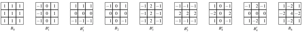
Figure 2. Basis functions for the 2D discrete cosine transform (not normalized).
III. SPECTRAL PREDICTOR,S
Our spectral predictorSgeneralizesL2andRto all possible configurations of 0 to 8 known samples and locations of the predicted sample in a 3×3 neighborhood. As in image compression methods based on discrete wavelet [16] and cosine transforms [17], we capitalize on the fact that the signal power is often heavily skewed toward low frequencies. In frequency transforms, this results in small, compressible high-frequency detail coefficients, whereas in predictive cod-ing “smooth” interpolants recover most of the low-frequency response, leading to small correctors for the missing high-frequency content.
In this section, we design as-smooth-as-possible interpolants for irregular sample configurations. We seek to eliminate or, when not possible, to minimize high-frequency responses in the interpolant. The resulting predictors and their sets of weights can be stored in a lookup table indexed by the mask of known and unknown values and the location of the predicted sample.
We build upon the work by Isenburg et al. [18], who use the Fourier transform to predict the geometry ofn-sided polygons to be “as regular as possible” given m<n known vertices. They express the vertex coordinates of the polygon in the complex plane, apply the discrete Fourier transform (DFT) to this n-vector of consecutive vertex coordinates, set the highest n−m frequencies to zero, and compute the inverse transform to obtain the complex coordinates of the predicted vertices. Because the Fourier transform is linear, the unknown vertices can be expressed as a linear combination of the known vertices. By working out the mathematics of the forward and inverse Fourier transforms, one can a priori establish a set of weights for a given configuration (m,n) of known and unknown number of vertices (i.e. the weights are not dependent on the geometry of the known samples). Because Fourier frequencies come in pairs, this approach works well when m is odd as then the resulting weights are guaranteed to be real. One can show that the discrete cosine transform (DCT) can instead be used whenmis even. Lifting the DFT to higher dimensions, Isenburg et al. further showed that the
L1 predictor from Section II-A is in the spectral sense the optimal predictor (i.e. smoothest interpolant) for hypercube-like neighborhoods with one unknown sample.
A. Spectral derivation of L2and R
We begin by extending the general approach of Isenburg et al. to 3×3 neighborhoods to re-derive the bi-Lorenzian and radial predictors and show that they are optimal. We will make
use of the two-dimensional (orthonormal) discrete cosine basis
{u(x)u(y),s(x)u(y),u(x)s(y), s(x)s(y),c(x)u(y), u(x)c(y), s(x)c(y),c(x)s(y),c(x)c(y)}
wherexandyvary over the domain {−1,0,+1}of our 3×3 neighborhood, and where
u(x) =
1
3, s(x) =
2 3sin
1
3πx
, c(x) =
2 3cos
2
3πx
The cosine basis is shown un-normalized in Fig. 2. We unfold the 3×3 matrix into a single 9-dimensional vector
b =fi−1,j−1 fi,j−1 fi+1,j−1 ··· fi+1,j+1
T
of sample values, and write the cosine basis as a 9×9 orthogonal matrix
B, where the columns of B are the basis functions. Then the forward discrete cosine transform is simply x=BTb, with x
being the DCT coefficients in order of increasing frequency. To extend the ideas of Isenburg et al. from 1D to 2D, we must rank the basis functions by increasing frequency. The cosine basis formulation gives us pairs of frequencies (ωx,ωy)for the horizontal and vertical direction, which must
be consolidated into single frequencies. We approach this by deriving the cosine basis through eigenanalysis of the symmetric combinatorial graph LaplacianL (also called the Kirchoff matrix [19])
li j= ⎧ ⎨ ⎩
deg(i) −1
0
ifi=j
ifi and j are adjacent otherwise
(4)
where we consider the graph formed by the 3×3 neighbor-hood in isolation, with vertical and horizontal edges between adjacent samples. Here deg(i) denotes the degree or number of neighbors of a samplei, e.g. deg(i)is 2 for corner samples, 3 for edge samples, and 4 for face samples. As noted by Strang [20], the eigenbasis of the (un-normalized, symmetric, positive semidefinite) Laplacian coincides with the discrete cosine basis (the DCT-2 basis), and the eigenvalues {λi} of
L are of the form
λ=22−cosωx−cosωy
=4sin2ωx 2 +sin
2ωy 2
(5)
withω=π3k,k∈ {0,1,2} for 3×3 neighborhoods. It follows that the eigenvalues of L are (0,1,1,2,3,3,4,4,6). Thus, larger eigenvaluesλ correspond to higher frequenciesω, and from here on we will use the terms eigenvalue and frequency interchangeably. We will further use Bλ to denote the eigen-vector (i.e. basis function) with corresponding eigenvalue λ, andBxλ andByλ to distinguish pairs of eigenvectors with equal eigenvalues (Fig. 2).
M= 10 00 00 00 00 01 00 00 00
? 35 2 5
PT= 10 √02 5
0 1 √ 5
0 0
0 0
0 0
0 0
0 0
0 0
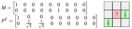
Figure 3. Example mask matrixM, interpolation matrixP, and weightsW.
similarly to Isenburg et al., we set the highest frequency response x6 to zero and solve for the unknown sample as a linear combination of the m=8 known samples, which results in the weights given in (2) and (3) for corner and center predictions.
B. The general case: Irregular sample configurations
Whenm<8, a similar strategy is possible by zeroing 9−m
of the highest frequencies. However, we may need to resolve two issues:
(1) The 9−mfirst basis functions may not form a basis for the set of known samples, e.g.{B0,Bx1,By1}is not a basis for b=fi−1,j−1 fi,j−1 fi+1,j−1 0 ··· 0
T
. (2) In situations when only one ofBxλ andByλ is needed (e.g.
when exactly two samples are known, as in Fig. 3), we may reduce the total frequency response by choosing a linear combination ofBxλ andByλ.
LetM be an m×n mask matrix that extracts themknown samplesMbfromb, i.e. each row ofM has a single one entry and remaining zeros. We wish to solve the underconstrained systemMBx=Mb for xwith as many high frequencies of x
zeroed as possible. This can be done via linearly constrained least-squares methods, which involves symbolic inversion of an(m+n)×(m+n)matrix. We show here how to accomplish the same goal via inversion of a smallerm×mmatrix.
We first must find an m-dimensional basis for Mb by selecting from or combining the n>m column vectors MB; any excluded vector from MB will implicitly have its cor-responding frequency response zeroed. Our approach is to incrementally construct an n×m interpolation matrixP that linearly combines vectors from MB such that MBPy=Mb
is a fully constrained system of m equations, with Py=x. We achieve this by adding to P columns that select basis functions from MB in order of increasing frequency λ. If a basis function projected onto the space of known samples is redundant (linearly dependent) with respect to the partially constructed basis, we exclude it and consider the next basis function. When we encounter an eigenspace, i.e. two basis functions with the same eigenvalue, one of three situations arises: (1) The whole eigenspace is redundant, and we exclude it. (2) The whole eigenspace is nonredundant, and we include it. (3) The eigenspace is partially redundant, in which case we first “rotate” the eigenspace by an angle θ to make one of the rotated and projected basis functions redundant. (Note that any rotation of an eigenspace preserves eigenvalues and orthogonality with the rest of the basis.) This leaves a nonredundant basis function Bθλ =cos(θ)Bxλ+sin(θ)Byλ and we add toPa column that has cos(θ)and sin(θ)in the rows corresponding to Bx
λ and Byλ. The effect of this rotation is to “align” the basis function with the spatial configuration of
known samples. One can show that this rotation leads to the minimal total frequency response||x||.
We may now compute x=P(MBP)−1Mb using matrix inversion. We are, however, not interested in the frequency responsexbut in the weights of the known samplesMb. Hence we apply the inverse DCT toxand computeBx=W b, where
W is then×nweight matrixW=BP(MBP)−1M. That is, row iofW gives the weights for interpolating an unknown sample
bifrom its known neighbors:bi=∑jwi jbj. Of course, ifbi is
a known sample, only wii=1 is nonzero.
We have implemented this method symbolically in Mathe-matica. A complete code listing is found in Appendix I. Com-puting exact weights W for all neighborhood configurations results in 41 unique weights in the range [−4,+4] that are predominantly integers and otherwise rationals (see [14] for a complete list of weights). In Appendix IV we prove that our weights always add to one, which makes our scheme affine invariant. Another desirable feature of spectral interpolation is self-interpolation: interpolating a sample s from a set S and then interpolating t from T =S∪ {s} yields the same result as interpolating t directly from S. We prove this property in Appendix V.
C. Choosing a neighborhood
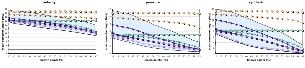
Via translation we can form nine 3×3 neighborhoods around each predicted sample p. Depending on the config-uration of known samples it is not immediately clear which neighborhood to predict from. We propose training the com-pressor on the given data set: each of the 9×28 predictors is exercised on each sample and receives a ranking based on the mean error it makes. This short ranking is transmitted before compression begins and determines the choice of predictor. In Fig. 4 we show using random sampling of two data sets that our approach improves upon several alternatives that we have explored, including the neighborhood centered at p and the mean or the median of all nine predictions. For calibration, we also report the results for the best (lowest residual) of the nine neighborhoods (which unfortunately is not available to the decoder), as well as the mean and median of constant (single-value) and L1 prediction.
IV. APPLICATIONS OF SPECTRAL PREDICTION Our spectral predictor is particularly useful in applica-tions where standard compression techniques, e.g. based on wavelets, are not practical, such as for encoding data sets with irregular domains due to manual or automatic extraction, in-painting, selective updates, adaptive sampling, or range queries that extract those samples whose values fall within an interval. Irregular sample configurations also arise when the data is traversed in other than scanline order, or in mesh compression, where the domain connectivity is inherently irregular. For lack of space, we here consider only a few of these applications.
velocity
0 2 4 6 8 10 12 14 16 18 20 22
10 15 20 25 30 35 40 45 50 55 60 65 70 75 80 85 90 95 known points (%)
mean corrector length (bits)
pressure
0 2 4 6 8 10 12
10 15 20 25 30 35 40 45 50 55 60 65 70 75 80 85 90 95 known points (%)
mean corrector length (bits)
synthetic
0 2 4 6 8 10 12 14 16
10 15 20 25 30 35 40 45 50 55 60 65 70 75 80 85 90 95 known points (%)
mean corrector length (bits)
Const ant Median Const ant Mean L1 Median L1 Mean Spect ral Median Spect ral Mean Spect ral Cent ered Spect ral Trained
Figure 4. Predictor quality vs. average number of known points in the 3×3 neighborhood. The shaded area bounds the best and worst spectral prediction.
0% 10% 20% 30% 40% 50% 60% 70% 80% 90% 100%
Viscocity Pressure Velocity Diffusivity Vorticity
normalized mean prediction error
Paeth Median L1 L2
(a) Scanline transmission
0 2 4 6 8 10 12 14 16 18 20
Viscocity Velocity Diffusivity Vorticity
mean corrector length (bits)
Bilinear Hybrid Spectral
(b) Progressive refinement
0 1 2 3 4 5 6 7
1000m 1001m 1003m
mean corrector length (bits)
Median Mean Spectral
(c) Isocontouring
Figure 5. Prediction results for three different applications.
A. Scanline transmission
The most straightforward way to compress regularly gridded data is to make a scanline traversal, e.g. row-by-row from bottom to top and from left to right within each row. We here compare our bi-Lorenzian L2 predictor with other scanline predictors proposed for image compression: the Paeth predic-tor [12] used in the PNG image format [5], the median pre-dictor used in JPEG-LS [4], and theL1Lorenzo predictor [13] used by Lindstrom and Isenburg [9]. All exceptL2 predict a sample from the same set of three neighbors (Fig. 1(a)).
In order to apply L2 in a scanline traversal, two rows of previously coded samples must be maintained (Fig. 7(a)). To bootstrap the predictor, one may use lower-dimensional Lorenzo prediction to first recover domain boundaries. Alter-natively, one may use the spectral predictor for partially known neighborhoods described in Section III.
Fig. 5(a) shows the results of predicting multiple 2D slices of the single-precision floating-point scalar fields shown in Fig. 6 obtained from a fluid dynamics simulation [1]. On high-precision data like this, L2 often offers substantially better prediction than predictors that use smaller stencils. The benefit of a larger stencil comes at the expense of higher sensitivity to quantization, however, due to accumulation of per-sample errors and larger (in magnitude) weights. Analysis shows that the prediction error due to quantization is three times larger for L2 than for L1 (see Appendix III). Hence L2 generally performs worse than L1 on low-precision data such as 8-bit images.
B. Progressive refinement
Often, data sets are transmitted progressively, doubling the resolution inxandyafter each refinement. The missing values within a refinement level may be transmitted in scanline order, as shown in Fig. 7(b), which results in three 3×3 neigh-borhood configurations from which samples are predicted (Fig. 7(b–d)).
We consider three predictors for the face sample (Fig. 7(c)): bilinear interpolationBof corner samples (Fig. 1(d)), spectral predictionSf (Fig. 1(f)), and a hybrid predictorH (Fig. 1(e)) that first linearly interpolates the unknown neighbors at the vertical and horizontal edges from their immediate neighbors to fill the neighborhood and then predicts the face point using radial prediction R. Note that both B and H are instances of spectral prediction that simply ignore some of the known neighbors. For the edge points, B and H resort to linear interpolation of corner points for prediction (since no other reasonable non-spectral predictor is available), while our spec-tral predictor is able to make use of all decoded samples (Figs. 1(g) and 1(h)).
Fig. 5(b) illustrates the advantage of using all known neighboring samples in the prediction. Sf offers in all cases
(a) Density (b) Pressure (c) Diffusivity (d) Viscocity (e) Vorticity
Figure 6. (a–d): Interval-volume renderings of several of the 3D scalar fields used in our experiments. (e): Close-up of the 1025×5000 2D vorticity field.
◦ ◦ ◦ ?
◦ ◦ ◦ ◦ ◦ × ◦ ◦ ◦ ◦ × × × × ×
(a)
• • •
◦ ◦ ◦ ?
• ◦ • ◦ • ◦ ◦ ◦ ◦ ◦ • ◦ • ◦ •
(b)
• •
◦ ?
• ◦ •
(c)
• •
◦ ◦ ?
• ◦ •
(d)
• ? •
◦ ◦ ◦ • ◦ •
(e)
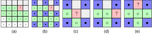
Figure 7. (a) L2 footprint (circles) maintained during scanline traversal.
(b) Coarse-resolution (solid) and fine-resolution (hollow) processed samples in a hierarchical traversal. Within each level of resolution, scanline traversal is used, resulting in three predictor stencils: (c) face, (d) vertical edge, and (e) horizontal edge sample.
C. Isocontouring
In many scientific, engineering, and medical applications, regularly sampled volumetric scalar fields are visualized in terms of isosurfaces. For instance, a remote viewer may wish to see the isosurfaceS(t)formed by all points at temperaturet
or to explore the familyS(T)of isosurfaces with temperatures in a rangeT= [tmin,tmax]. Instead of transmitting the geometry
ofS(t)or some compressed form of its animation, it is often more effective to transmit the minimal subset of scalar values needed to reconstruct the single isosurfaceS(t)or family of isosurfaces S(T) [21]. To satisfy this query, one needs to transmit not only the samples with values inT, but also some of their neighbors to obtain a complete “scaffold” around the surface. In a scenario where the remote user later decides to extend T to a larger interval, compression and incremental transmission of the subset of additional samples would often be preferable over complete retransmission. For both initial and incremental transmission, it is not obvious how to predict the irregular subset of sample values using traditional means. Although isocontouring of 3D volume data is a more common task than isocurve extraction from 2D fields, we focus here on the 2D case as it allows for straightforward application of our 3×3 predictor. Aside from the higher memory usage of the lookup tables needed by a 3D spectral predictor, the generalization from 2D to 3D is largely straightforward.
Our approach is based on the traversal, identification, and transmission of the minimal subset of samples that completely determine the isocontour requested by the client. We use an isocontour extraction method similar tomarching cubes[22], but avoid traversing the entire 2D data set for each requested isocontour. Rather, we assume that a pre-computed set of seeds is available to the encoder from which it is possible to recover the isocontour [23]. The benefit of this seed set is that it allows visiting only thosecellsintersected by the isocontour. A cell is the rectangular region in the 2D grid between four neighboring
samples, which are pairwise joined bylinks(edges in the grid). We call the links intersected by the contour sticks, i.e. the two sample values of a stick bracket the given isovalue. As is common, the vertices of the isocontour are placed on the sticks by linearly interpolating the function values at the stick endpoints and solving for the position where this interpolant equals the isovalue.
The encoder and decoder perform the same traversal, hence we discuss them together. They both store in memory the surrounding sample values that determine the isocontour. Our implementation uses a quadtree as a sparse data structure for storing a mask of known samples and their values. This structure provides fast, adaptive storage, while maintaining spatial relationships between the samples.
1) Compression Algorithm: Our compressor encodes
iso-contours one component at a time. For each component, it begins with a seed stick and encodes its two sample values (A, B from Fig. 8). The encoder then follows the isocontour until it exits the domain of the data set or returns to the seed stick. During this traversal, we enter a cell through a stick and exit through another. While the isocontour never bifurcates, it is possible for a cell to have four sticks, in which case the contour passes through the same cell twice.
The two samples at the entrance stick are known by both encoder and decoder, however the other two samples of the cell (C and D in Fig. 8) may not be known by the decoder. This leads to the following three cases when entering a cell:
(1) Only the two samples from the entrance stick are known. To determine the exit stick, we must first decide which of the samplesC and D to encode first; it is possible that only one of them is needed to trace the isocontour. We use our spectral predictor to produce estimates C
and D for the remaining samples. If AC is a stick, we encode/decode C and continue to the next case below. Otherwise, we perform the same test forBDand transmitDif the test passes. If neither link is estimated to be a stick, we encodeCorDdepending on which is closest to the intersection point between the isocontour and the entrance stick. This simple heuristic works well in practice, and often identifies the correct exit stick. (2) Three samples are known, including the two samplesA
andBfrom the entrance stick. Without loss of generality, we assume thatC is the other known sample. If AC is a stick, then it becomes the exit stick. Otherwise we encode/decodeD, and determine through which link of
B
D C
A
Figure 8. Example 2D cell. The entrance stick is shown in green, the already encoded samples in blue, and the traversed part of the isocontour in red.
B
D C
A B
D C
A
Figure 9. Ambiguous case in 2D isocontouring (x-cells).
(3) All four samples are known. If in addition to the en-trance stick the cell contains only one more stick, this becomes the exit stick (nothing needs to be encoded). Otherwise, all four links are sticks, and the contour passes through the cell twice. We call such cellsx-cells. Without information on the behavior of the continuous function in the interior of the cell, there are two pos-sible and equally valid interpretations of how to trace the isocontour (see Fig. 9). Several criteria have been proposed for resolving such ambiguities (e.g. [24], [25]), and we leave it up to the client to interpret such cells. However, in order to visit all samples needed by the isocontour, the encoder/decoder must agree on which cell to visit next. For simplicity, we use our heuristic above and exit through the link closest to the entrance vertex (intersection). Note that this choice affects only the order of samples encoded, i.e. it has no impact on which cells are traversed or which samples are needed to extract the isocontour.
To encode the value of a sample, we use spectral prediction and the residual coder from [9]. As discussed in Section III-C, we have freedom in positioning the neighborhood around the predicted sample. From the nine possible neighborhoods, we use as heuristic the one containing the largest number of known samples (though training the predictor, as in Section III-C, is also possible).
To bootstrap the decoder, we transmit with each component a start seed in the form of a stick. This stick is encoded as the location of its left-most, bottom-most sample, and a single bit indicating its orientation (horizontal or vertical). If no nearby samples are available, we use the isovaluewas prediction of the first sample f0. The other seed sample, f1, which together with f0 must bracketw, is then predicted as f1=2w−f0.
It is important to point out that our approach never transmits the value of a sample more than once. If a sample was previously encoded with an isocontour, it will be available locally to the client for extraction of subsequent isocontours.
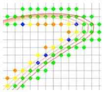
Figure 10. Close-up of a sequence of transmitted isocontours. The set of samples transmitted with each isocontour is shown in a separate color.
(a) small (b) medium (c) large (d) very large
Figure 11. Four sets of isocontours from the synthetic circle data set. From left to right, the step between isovalues is doubled. Each isocontour and the samples they depend on are shown in a different color. As is evident, fewer samples are transmitted for more closely spaced isocontours.
2) Results: We have evaluated our isocontour compressor on three data sets: an isotropic distance map with circles as isocontours (Fig. 11), a 1,025×5,000 vorticity scalar field from a numerical hydrodynamics simulation by Miller et al. [26] (Fig. 6(e)), and the 16,385×16,385 Puget Sound 16-bit precision terrain surface [27]. The first two data sets are stored in single (32-bit) precision floating point.
Though it is common to measure isocontour compression in terms of the number of bits per generated isocontourvertex
(bpv) transmitted, we will also evaluate our method in terms of number of bits per function sample(bps).
When our implicit technique is used to compress a single isocontour, it generally does not perform as well as methods that explicitly compress the isocontour representation directly. This is to be expected, as we encode information sufficient to extract a range of isocontours and to evalute the function over a subset of the domain. For the 32-bit floating-point circle data set, our method compresses large isocontours to 17.13 bits per vertex, equivalent to 12.10 bits per sample. For this same isocontour, 4.2 neighbors are available on average for prediction. Because locally the isocontour is mostly “straight,” the neighborhood configuration is often such that the spectral predictor has to resort to 1D linear extrapolation, which is not a particularly powerful predictor.
0 5 10 15 20
1 2 3 4 5 6 7 8 9
Small Increment Medium Increment
Large Increment Disjoint
Figure 12. Compression in bits per vertex for each set of isocontours from Fig. 11. The horizontal axis corresponds to subsequent isocontours transmitted (from left to right). The graph shows that when isocontours are closely spaced together fewer samples need transmission and better prediction is possible.
“large” data set has almost the same sample/vertex ratio as the individual isocontour, but its prediction is improved by having nearby samples from previously transmitted isocontours. As long as the new isocontour is nearby already decompressed data, our technique offers improvement. The compression for the “very large,” “large,” “medium,” and “small” examples is 17.28, 13.64, 6.49 and 4.13 bits per vertex, respectively.
As a result of the way the samples are predicted, the order in which isocontours are encoded affects the compression ratio. For sets of disjoint isocontours the order has no influence on compression, but when isocontours are close the order does matter. To illustrate this point, we compressed the “medium” spaced set of isocontours in different orders. In the worst case, the first half of the isocontours are transmitted in an order where there is no overlap, even though there are enough nearby points to help prediction, resulting in compression similar to the “large” example. The second half of isocontours overlap those from the first half, and hence few additional samples are transmitted. Here 8.0 neighbors are available on average, which allows near perfect prediction at only 0.8 bits per vertex. The average cost across all isocontours is in this case 8.22 bpv. When instead the isocontours are transmitted in order of increasing isovalue, there is sufficient overlap for consistently good prediction, resulting in only 6.49 bits per vertex. Note, however, that the client may not be at liberty to choose this order as it may be dictated by the user.
We also evaluate our method on two differently spaced sets of nine isocontours each from the “vorticity” data set (Fig. 6(e)). The “large” isovalue range from this data set is twice as wide as the “medium” range. We achieve on average 16.6 bits per vertex on the “large” example, and 12.08 on the “medium.” By comparison, compressing a single isocontour requires 34.0 bpv. As in our other single-isocontour examples, the transmitted samples are often predicted poorly only via extrapolation along the isocontour, resulting in a cost similar to encoding each 1D stick intersection using a raw 32-bit floating-point representation.
As before, the initial overhead of our technique can be amortized over several isocontours, and again the transmission order matters (see Table I). We have observed in all cases that if the objective is to encode all the samples in a range, it is best to encode them sequentially (e.g. in order of
increas-TABLE I.
DEPENDENCE OF COMPRESSED FILE SIZE ON ISOCONTOUR
TRANSMISSION ORDER FOR THE MEDIUM-DENSITY2DCIRCLE EXAMPLE. ISOCONTOURS ARE NUMBERED BY INCREASING,EQUISPACED ISOVALUE.
Transmission Order File Size 1,2,3,4,5,6,7,8,9 32537 1,3,5,7,9,2,4,6,8 41214 1,5,9,3,7,2,4,6,8 44599
ing isovalue) rather than hierarchically (e.g. by interleaving isocontours). In the sequential encoding we observed a 20% improvement over the hierarchical encoding. The improvement is entirely dependent on the accuracy of prediction since the same set of samples is eventually transmitted. In sequential transmission each point is predicted from a close-to-full stencil (7 to 8 neighbors), while hierarchical encoding is relegated to use sparsely populated stencils (4 neighbors on average) for half of the isocontours.
We end this section by reporting experiments of extract-ing isolines from the Puget Sound terrain surface. We first extracted an isocontour at 1000 m elevation and predicted all necessary samples, then incrementally transmitted missing values for isocontours at 1001 m and 1003 m, resulting in an average number of known neighbors of 5.13, 5.42, and 5.41, respectively. Since samples are often not available for predictors like L1 to be applied, we compare our spectral predictor with predictions based on the mean and median sample value in a 3×3 neighborhood centered on the predicted sample. We observed consistent reduction in corrector bit length (13–22%) using the spectral predictor, even for this lower-precision data set (Fig. 5(c)).
V. CONCLUSIONS
We have described two new predictors, the bi-Lorenzian
L2 and the radial R, which predict the value of a sample f from eight values in a 3×3 neighborhood of which f is the corner (for L2) or the center (for R). More importantly, we propose the spectral predictor S, which extends L2 andR to all configurations of 0 to 8 known samples and locations of f
in a 3×3 neighborhood. We argue thatS is the best predictor from a 3×3 neighborhood, provide a strategy for selecting the most promising neighborhood that contains f, and demonstrate the benefits of S over competing predictors in three simple applications.
APPENDIXI IMPLEMENTATION
Listing 1 is a Mathematica 5.0 implementation of the spec-tral interpolator. Given a Laplacian matrixL that represents the stencil from which predictions are made and a vector S
that specifies which samples are known (1) and unknown (0), the weight matrixW is computed. The bi-Lorenzian weights, e.g., are obtained by weight[{0, 1, 1, 1, 1, 1, 1, 1, 1}][[1]]. For completeness, the 3×3 Laplacian is included here, but it may be redefined for arbitrary stencils.
Listing 1. Mathematica code for computing spectral weight matrix.
Needs[ ” L i n e a r A l g e b r a ‘ O r t h o g o n a l i z a t i o n ‘ ” ]
(∗ L a p l a c i a n f o r 3 x3 s t e n c i l ∗)
l a p = {{ 2 , −1, 0 , −1, 0 , 0 , 0 , 0 , 0 }, { −1, 3 , −1, 0 , −1, 0 , 0 , 0 , 0 }, { 0 , −1, 2 , 0 , 0 , −1, 0 , 0 , 0 }, { −1, 0 , 0 , 3 , −1, 0 , −1, 0 , 0 }, { 0 , −1, 0 , −1, 4 , −1, 0 , −1, 0 }, { 0 , 0 , −1, 0 , −1, 3 , 0 , 0 , −1 }, { 0 , 0 , 0 , −1, 0 , 0 , 2 , −1, 0 }, { 0 , 0 , 0 , 0 , −1, 0 , −1, 3 , −1 }, { 0 , 0 , 0 , 0 , 0 , −1, 0 , −1, 2 }}
(∗ e i g e n b a s i s B o f L a p l a c i a n ∗)
b = T r a n s p o s e[ GramSchmidt [R e v e r s e[E i g e n v e c t o r s[ l a p ] ] ] ]
(∗ o r d e r e d e i g e n s p a c e i n d e x s e t s ∗)
e = S p l i t[
Range[Length[ l a p ] ] ,
Equal@@R e v e r s e[E i g e n v a l u e s[ l a p ] ] [ [{# #}] ] & ]
(∗ mask m a t r i x M( S ) ∗)
mask [ s ] : = S e l e c t[D i a g o n a l M a t r i x[ s ] , Norm[ # ]> 0 &]
(∗ add l i n e a r l y i n d e p e n d e n t c o l u m n s t o m a t r i x P ∗)
e x t e n d [ mb , {}, q t ] : = q t e x t e n d [ mb , p t , q t ] : = J o i n[
p t ,
S e l e c t[
RowReduce[
N u l l S p a c e[ p t . T r a n s p o s e[ mb ] ] . mb . T r a n s p o s e[ q t ] ] . q t ,
Norm[ # ]> 0 & ]
]
(∗ i n t e r p o l a t i o n m a t r i x P ( S ) ∗)
i n t e r p [ s ] : = Module[ {mb = mask [ s ] . b , p t},
For[ p t = {}; i = 1 , Length[ p t ] < Length[ mb ] , i ++ ,
p t = e x t e n d [ mb , p t , I d e n t i t y M a t r i x[Length[ s ] ] [ [ e [ [ i ] ] ] ] ] ] ;
T r a n s p o s e[ p t ] ]
(∗ w e i g h t m a t r i x W( S ) f o r s a m p l e s e t S ∗)
w e i g h t [ s ] : = Module[
{m = mask [ s ] , p = i n t e r p [ s ]}, b . p . I n v e r s e[m . b . p ] . m ]
APPENDIXII PREDICTORACCURACY
We here investigate the accuracy of the bi-Lorenzian (L2), edge (Sh), and radial (R) predictors for general (e.g.
non-polynomial) functions f. Without loss of generality, consider predicting f(0,0). If f is smooth or sufficiently densely sampled, we can approximate it well in the vicinity of the
predicted sample by a second order Taylor series expansiong:
gx,y=
2
∑
i=02
∑
j=0f(i,j)(0,0) i!j! x
iyj
where f(i,j) denotes the ith and jth partial derivative with respect to x and y, respectively. We then have as prediction error f(0,0)−p(0,0), where we express the prediction pas a weighted combination of samplesgx,y according to the given predictor weights. For the bi-Lorenzian predictor, the error is:
f(0,0)−2(g1,0+g0,1+g2,1+g1,2)
−4g1,1−(g2,0+g0,2+g2,2)
=f(2,2)(0,0)
Similarly, the edge predictor yields an error of 12f(2,2)(0,0)
and the radial predictor an error of 14f(2,2)(0,0). Thus, in the limit the radial predictor is four times as accurate as the bi-Lorenzian.
APPENDIXIII SENSITIVITY TONOISE
The sampled function often contains noise, either due to an imperfect acquisition process or due to errors stemming from limited precision and quantization. Assuming otherwise perfect prediction, we analyze how noise affects the accuracy of our predictors. We assume that each function value f(i,j)
involved in the prediction is perturbed by a small offset
δ(i,j)∈[−ε,+ε]uniformly distributed in this interval, which well models effects such as integer quantization. The square errorE2due to noise then reduces to:
E2=δ(0,0)−
∑
i∑
jw(i,j)δ(i,j)2
where w(i,j) is the predictor weight of sample f(i,j). We find the root mean square error via multiple integration of the
{δ(i,j)}over the domain[−ε,+ε]nof then-point stencil. For 3×3 neighborhoods, we obtain the RMS errors (expressed in multiples of ε) listed in Table II.
TABLE II.
NOISE-INDUCED ERRORS FOR SELECTED SPECTRAL PREDICTORS.
Stencil Sample Name Error /ε
2×1 corner constant
2 3 0.816
3×3 face radial
√
3 2 0.866
3×1 edge linear interpolation 11.000
3×2 edge 11.000
2×2 corner Lorenzo √2 3 1.155
3×1 corner linear extrapolation √21.414 3×3 edge edge predictor √31.732
3×2 corner 22.000
3×3 corner bi-Lorenzian 2√33.464
APPENDIXIV AFFINEINVARIANCE
weight matrixW =BP(MBP)−1M satisfiesW1
n=1n, where
1n is a vector ofnones.
Lemma 4.1: The first n-entry column of the interpolation matrixPequals [1 0 ··· 0]T.
Proof: It is well known that the first eigenvector of the LaplacianL is B0=√1n1n, with a corresponding unique
eigenvalueλ0=0. Since any nonempty sample set is linearly dependent on MB0, we always include it in the construc-tion of the basis MBP by setting the first column of P to [1 0 ··· 0]T.
Theorem 4.2: For any nonempty sample set,W1n=1n. Proof: Let v= [√n 0 ··· 0]T be anm-vector. Due to Lemma 4.1,Pv= [√n 0 ··· 0]T. Thus,BPv=√nB0= 1n. Further note thatMBPv=1m, and hencev= (MBP)−11m.
So 1n=BPv=BP(MBP)−11m=BP(MBP)−1M1n=W1n.
APPENDIXV SELF-INTERPOLATION
We here prove the self-interpolating property of our spectral interpolator: given a set of samples S and a superset T
interpolated fromS, it matters not whether additional samples are interpolated from S only or from T. In other words,
WTWS=WS, where we have used subscripts to distinguish
between weights computed from different sample sets. The proof begins with a lemma:
Lemma 5.1: For anyS⊆T, there exists a matrixXS,T such thatBPS=BPTXS,T.
Proof: The columns ofBPSform a basis for the columns of MT
S over the samples S, i.e. the columns of MSBPS span
the columns of MSMST =I. Since MTBPT is a basis for MTMTT, since ran(MTT)≥ran(MST), and since basis functions
are added in the same order to construct bases forS andT, we have thatBPT is also a basis for MST overS. As a result,
ran(BPT)≥ran(BPS), which implies that we can writeBPSas
linear combinations of BPT, i.e. there is a matrix XS,T such
thatBPS=BPTXS,T.
Theorem 5.2: For anyS⊆T,WTWS=WS.
Proof: LetWS=BPS(MSBPS)−1MSbe the weight matrix
for the sample setS. We have:
WTWS=BPT(MTBPT)−1MTBPS(MSBPS)−1MS
=BPT(MTBPT)−1MTBPTXS,T(MSBPS)−1MS
=BPTXS,T(MSBPS)−1MS
=BPS(MSBPS)−1MS
=WS
ACKNOWLEDGEMENTS
This work was performed in part under the auspices of the U.S. Department of Energy by University of California, Lawrence Livermore National Laboratory under contract W-7405-Eng-48.
REFERENCES
[1] A. W. Cook, W. H. Cabot, P. L. Williams, B. J. Miller, B. R. de Supinski, R. K. Yates, and M. L. Welcome, “Tera-scalable algorithms for variable-density elliptic hydrodynamics with spectral accuracy,” in ACM/IEEE Supercomputing, 2005, p. 60.
[2] G. W. Larson, “LogLuv encoding for full-gamut, high-dynamic range images,” Journal of Graphics Tools, vol. 3, no. 1, pp. 15–31, 1998.
[3] D. F. Maune, Digital Elevation Model Technologies and
Ap-plications: The DEM Users Manual. American Society for
Photogrammetry and Remote Sensing, 2001.
[4] M. J. Weinberger, G. Seroussi, and G. Sapiro, “The LOCO-I lossless image compression algorithm: Principles and standard-ization into JPEG-LS,”IEEE Transactions on Image Processing, vol. 9, no. 8, pp. 1309–1324, 2000.
[5] G. Roelofs,PNG: The Definitive Guide. O’Reilly, 2003, http: //www.libpng.org/pub/png/book/.
[6] C. Touma and C. Gotsman, “Triangle mesh compression,” in
Graphics Interface, 1998, pp. 26–34.
[7] V. Engelson, D. Fritzson, and P. Fritzson, “Lossless compression of high-volume numerical data from simulations,” in Data
Compression Conference, 2000, pp. 574–586.
[8] P. Ratanaworabhan, J. Ke, and M. Burtscher, “Fast lossless com-pression of scientific floating-point data,” inData Compression Conference, 2006, pp. 133–142.
[9] P. Lindstrom and M. Isenburg, “Fast and efficient compression of floating-point data,”IEEE Transactions on Visualization and Computer Graphics, vol. 12, no. 5, pp. 1245–1250, 2006. [10] H. Kobayashi and L. R. Bahl, “Image data compression by
predictive coding I: Prediction algorithms,” IBM Journal of Research and Development, vol. 18, no. 2, pp. 164–171, 1974. [11] E. H. Feria, “Linear predictive transform of monochrome im-ages,”Image and Vision Computing, vol. 5, no. 4, pp. 267–278, 1987.
[12] A. W. Paeth, “Image file compression made easy,” inGraphics
Gems II, J. Arvo, Ed. San Diego: Academic Press, 1991.
[13] L. Ibarria, P. Lindstrom, J. Rossignac, and A. Szymczak, “Out-of-core compression and decompression of largen-dimensional scalar fields,” Computer Graphics Forum, vol. 22, no. 3, pp. 343–348, 2003.
[14] [Online]. Available: http://www.cc.gatech.edu/∼lindstro/data/ spectral/
[15] L. Ibarria, P. Lindstrom, and J. Rossignac, “Spectral predictors,”
Data Compression Conference, pp. 163–172, March 2007.
[16] C. Chrysafis and A. Ortega, “Efficient context-based entropy coding for lossy wavelet image compression,” in Data Com-pression Conference, 1997, pp. 241–250.
[17] G. K. Wallace, “The JPEG still picture compression standard,”
Communications of the ACM, vol. 34, no. 4, pp. 30–44, 1991. [18] M. Isenburg, I. Ivrissimtzis, S. Gumhold, and H.-P. Seidel,
“Geometry prediction for high degree polygons,” in SCCG, 2005, pp. 147–152.
[19] H. Zhang, “Discrete combinatorial Laplacian operators for digital geometry processing,” inSIAM Conference on Geometric Design, 2004, pp. 575–592.
[20] G. Strang, “The discrete cosine transform,” SIAM Review, vol. 41, no. 1, pp. 135–147, 1999.
[21] A. Mascarenhas, M. Isenburg, V. Pascucci, and J. Snoeyink, “Encoding volumetric grids for streaming isosurface extraction,”
in3DPVT, 2003, pp. 665–672.
[22] W. E. Lorensen and H. E. Cline, “Marching cubes: A high resolution 3d surface construction algorithm,” in Computer
Graphics (Proceedings of SIGGRAPH 87), vol. 21, 1987, pp.
163–169.
Symposium on Computational Geometry (SCG-97), 1997, pp. 212–220.
[24] G. M. Nielson and B. Hamanna, “The asymptotic decider: resolving the ambiguity in marching cubes,” inIEEE Visual-ization, 1991, pp. 83–91.
[25] C. Andujar, P. Brunet, A. Chica, I. Navazo, J. Rossignac, and A. Vinacua, “Optimal iso-surfaces,” Computer-Aided Design and Applications, vol. 1, no. 1–4, pp. 503–511, 2004. [26] P. Miller, P. Lindstrom, and A. Cook, “Visualizations of the
dynamics of a vortical flow,”Physics of Fluids, vol. 15, no. 9, p. S13, 2003.
[27] [Online]. Available: http://www.cc.gatech.edu/projects/large models/ps.html
Lorenzo Ibarriawas born in Barcelona, Spain, where he received his BS in computer science from the Polytechnic University of Catalonia. He did his graduate studies at the Georgia Institute of Technology, achieving a MS and PhD in computer science. His areas of interest are compression and computer graphics. Currently he is working at NVIDIA.
Peter Lindstromwas born in Sweden and has resided in the U.S.
since 1990. He received a PhD in computer science from Georgia Institute of Technology in 2000, and holds BS degrees in computer science, mathematics, and physics from Elon University. He joined Lawrence Livermore National Laboratory in 2000, where he is a computer scientist and project leader. His primary research interests are in scientific visualization, data compression, mesh simplification, geometric and multiresolution modeling, and out-of-core techniques. Dr. Lindstrom is a member of ACM and IEEE. He has served on 15 international program committees, and has published over 30 articles.
Jarek Rossignacwas born in Poland and grew up in France. He
received a PhD in electrical engineering from the University of Rochester, NY, in 1985. Between 1985 and 1996, he worked at the IBM T.J. Watson Research Center in Yorktown Heights, NY, where he served as Senior Manager and as Visualization Strategist. In 1996, he joined the Georgia Institute of Technology, Atlanta, GA, where he served as Director of the GVU Center and is Full Professor in the College of Computing. His research focuses on the design, simplification, compression, and visualization of highly complex 3D shapes, structures, and animations.