Dickel

GROWTH AND SURVIVAL OF EUCALYPTUS GRANDIS — A

STUDY BASED ON MODELLING LIFETIME DISTRIBUTIONS

Meike Dickel

,

Heyns Kotze

,

Klaus von Gadow

Walter Zucchini

1_{Research Assistant, Christian-Albrechts-University Kiel, Germany}

2_{Komatiland Forests Pty. Ltd., Nelspruit, South Africa}

3_{Professor Emeritus,}∗_{Principal contact, Georg-August-Universit¨at G¨ottingen, Germany}

4_{Professor, Georg-August-Universit¨at G¨ottingen, Germany}

Abstract.The objective of this study is to analyse the density-dependent dynamics of growth and

mor-tality in an unthinned Eucalyptus grandis spacing experiment on a homogenous site in Zululand/South Africa. Specifically we propose models that describe how the (log) basal area develops in unthinned stands. Our data clearly indicate that mortality varies enormously with planting density. We therefore develop and investigate models that explicitly take mortality into account. To do so we first model the conditional distribution of log basal area as a function of age and the number of trees that are concurrently alive. The last of these covariates is generally unknown in advance, which would seem to render it inapplicable for the purpose of modeling the distribution of future basal area. We show how it is nevertheless possible to estimate the distribution of the number of surviving trees from the available data, and thereby to ‘integrate out’ the effect of this random variable in order to estimate the (unconditional) distribution of the log basal area for each planting density. This is achieved by fitting Weibull distributions to the lifetimes of the trees in the four available plots. A number of different models for the log basal area are compared.

Our estimates indicate that the distribution of the future basal area in an unthinned Eucalyptus gran-dis forest is not independent of the planting density, within the range of the experimental densities investigated in this study. Our results provide clear evidence that planting density has strong and long-lasting effects on basal area. Furthermore the estimates indicate that these effects persist for at least 40 years and that, even after length of time, the rate of convergence to a common condition is very slow.

Keywords: Planting density, spacing experiment, Weibull distribution, basal area growth

1

Introduction

The effect of planting density on the growth and sur-vival of trees has been the subject of numerous studies. Neighbouring trees compete with their crowns as well as their roots for the available growing space. To sur-vive in a competitive environment a tree must build up and maintain phytomass in order to access resources in the occupied growing space (Matyssek, 2003). Tree den-sity affects the spatial distribution of light and temper-ature, and the availability of moisture and nutrients in a forest. Tree diameter growth is especially sensitive to changes in density. This effect was first demonstrated by Craib (1939) in an analysis of a South AfricanCorrelated

Curve Trend(CCT)-spacing trial.

The CCT experiment is a classic spacing trial designed to predict the growth in plantations of various species of

pine and eucalyptus for a wide range of planting densi-ties, varying between extremely dense (2965 stems per ha) and free growth (124 stems per ha). The majority of these CCT experiments were devised by O’Connor (1935) and initiated in 1936 and 1937. The typical CCT experiment consists of 18 plots, covering 0.04 ha each, some with up to four replications. Nine of the 18 plots were left unthinned, the other nine were subjected to various thinning regimes. Detailed descriptions of the design and analysis of the CCT studies were published by Marsh (1957), O’Connor (1960), Burgers (1976), Van Laar (1982), Bredenkamp (1984), Gadow (1987) and Gadow and Bredenkamp (1992). The effects of site qual-ity and stand densqual-ity on tree growth may be confounded. Thus, controlled experiments on a uniform site are use-ful if the aim is to study the effect of density on tree growth.

The objective of this study is to analyse the density-dependent dynamics of growth and mortality in four ex-perimental plots planted at different spacings on a homo-geneous site. Particular emphasis will be placed on es-timating the (unconditional) distribution of stand basal area using a model that explicitly takes account of the probability of tree survival.

2

Material and Methods

This section presents the complete dataset used in this study and explains the modelling approach and the methods of model evaluation.

2.1 The dataset The material used in this study was derived from theEucalyptus grandisspacing experiment

“Langepan” which was established in September 1952

on the coastal plain of KwaZulu-Natal in South Africa, located at 28◦36’ S and 32◦13’ E. The altitude is about 60m above sea level. The mean annual rainfall on the ex-perimental site is 1400mm, of which about 70% falls dur-ing the months of October to April. The coastal plain is an elevated marine platform, which consists essentially of a thick deposit of wind-borne sand. The sands are acidic and poor in organic matter due to rapid decom-position in the moist sub-tropical climate and the aero-bic condition of the surface soils. The moisture storage capacity is very low, but this shortcoming is moderated by great rooting depth. The mean annual temperature is 21.8◦C. Frost is virtually unknown along the coastal plain.

The design of the Langepan experiment is a modifi-cation of the standard CCT spacing experiments which were planted throughout the forestry regions of South Africa. The most important modification is the very high planting density of 6726 trees per ha in Plot 1. The Langepan experiment is a randomized complete block design with three blocks and twenty treatments. Twelve of these are unthinned spacing treatments, representing the so-called basic series. The remaining eight treat-ments were subjected to different types of thinnings and are known as the thinning series. Additional detail is given by Bredenkamp et al. (2000). Currently only one of the original three blocks remains. Four plots of the

basic series, which are still intact, were selected for the

present study. Each plot covers an area of 0.04047 ha and is surrounded by a buffer strip (30m around each measurement plot) which is subject to the same treat-ment as the plot.

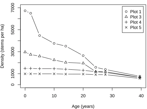
The complete dataset used in this study is presented in Table 1. For analysis standardised data per ha were used. The number of surviving trees per ha are displayed in Figure 1.

0 10 20 30 40

0

1000

3000

5000

7000

Age (years)

Density (stems per ha)

Plot 1 Plot 3 Plot 4 Plot 5

Figure 1: Observed density (stems per ha) as a function of age.

2.2 Modelling Approach One of the traditional methods used in the analysis of forest growth and tree survival is based on the state-space approach described by Garc´ıa (1994), where the system is characterized by a set of state variables which are assumed to be known at a given initial stage; transition functions are used to project all or some of the state variables to future stages. In selecting the state variables, the principle of parsimony must be taken into account. This means that the model should be the simplest one among alternative models which are consistent with the dynamics of the biological system (Milsum, 1966; Vanclay, 1995; Gadow, 1996; Burkhart, 2003).

In forests which are thinned ahead of natural mor-tality, dominant height and stand basal area (G_i) may be sufficient for estimating the system state at a given age (Pienaar and Turnbull, 1973; Decourt, 1974; Garc´ıa, 1988). In unthinned forests, especially those which are planted at high densities, it has been found to be nec-essary to include tree mortality, maximum density or the number of surviving trees (N_i) per unit area (Am-ateis et al., 1995; ´Alvarez-Gonz´alez et al., 1999; Garc´ıa, 2003; Di´eguez-Aranda et al., 2006; Castedo-Dorado et al., 2007).

The Langepan trial is an unthinned spacing

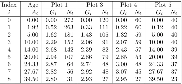
Table 1: The observations. Age (A_i) refers to years after planting, N_i the number of surviving trees, andG_i the basal area (m2_{) in the 0.04047 ha plots.}

Index Age Plot 1 Plot 3 Plot 4 Plot 5

i A_i G_i N_i G_i N_i G_i N_i G_i N_i

0 0.00 0.00 272 0.00 120 0.00 60 0.00 40

1 1.92 0.52 263 0.33 111 0.22 60 0.12 40

2 5.00 1.62 181 1.43 105 1.32 59 5.00 40

3 10.00 2.29 152 2.06 91 2.07 59 10.00 40

4 14.00 2.68 142 2.39 82 2.43 57 14.00 39

5 20.00 2.94 107 2.86 79 2.85 53 20.00 39

6 24.33 2.87 64 2.74 48 3.00 48 24.33 37

7 27.67 2.82 56 2.92 48 3.07 45 27.67 37

8 39.50 2.80 31 2.93 27 2.95 27 39.50 23

of our data.

As a first approach for estimating basal area we use the linear form of two models that had been applied in the past, designated here as the “Schumacher” and “Rodr´ıguez-Soalleiro” models. Both models use age and initial basal area as explanatory variables. However, in an unthinned spacing experiment, especially one with high planting densities, basal area growth is strongly affected by tree mortality. We therefore introduce an al-ternative modeling approach which takes account of the number of surviving trees as an additional explanatory variable. The initial age and basal area are assumed to be known, but the number of trees that survive to a given age is a random variable whose distribution can be modelled, which we do using a binomial distribution. Although the initial number of live trees (N0) is known, the probability that a given tree will survive to the given age has to be estimated. We do this by assuming that the lifetime of the trees follows a Weibull distribution. The parameters of the Weibull distribution, which de-pend on N0, can be estimated (for each N0 seperately) using the method of maximum likelihood. In that way the second parameter of the binomial distribution (‘the probability of success’) becomes available. In turn this allows us to explicitly take into account the variability in the basal area that is attributable to the uncertainty regarding the number of trees that will survive. This source of variation is ignored if one simply uses the ex-pected number of trees that will survive in the model for basal area. The latter approach provides a model for the distribution of the basal area under the condition that (precisely) the expected number of trees survive. Our approach provides a model that takes account of all possible survival outcomes (except the case in which no trees survive); in other words it provides a model for the unconditional distribution of basal area.

2.2.1 Models for area growth Traditionally, basal area at time point i (G_i) is estimated as a function of age at time point i−1 (A_i−1), the basal area at time pointi−1 (G_i−1), and one or two other covariates. We denote this as the “initial approach”. The approach pro-posed here, which we will refer to as the “alternative approach”, is to allow the distribution of basal area to depend on the number of surviving trees at time point i. This number is of course unknown in advance but, as was indicated above, its distribution can be estimated. For the estimation of basal area interval data of succes-sive measurements are used, starting from the age at planting.

Initial approach: Models that do not take ac-count of survival

A straight-forward model to estimate basal area is an age-related model, which was first proposed by Schu-macher (1939):

log(G_i)−log(G_i−1)

A_i−1

A_i =α1

1−Ai−1 A_i

(1)

One further model was proposed by Rodr´ıguez-Soalleiro et al. (1995):

log

G_i−G_i−1

A_i−A_i−1

=α0 + α1log(Gi−1) + α2log(Ai−1) (2)

Alternative approach: Models that involve the number of surviving trees

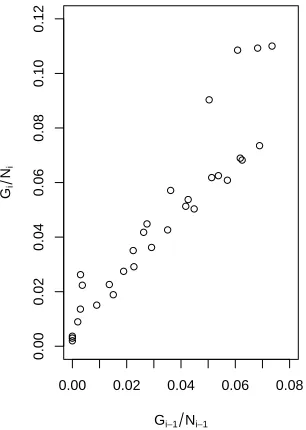
We begin by noting (see Figure 2) that there is an ap-proximately linear relationship between G_i−1/Ni−1 and

age, A2_i. The latter was included following an analysis of the residuals of the model without this term. The resulting model is

0.00 0.02 0.04 0.06 0.08

0.00

0.02

0.04

0.06

0.08

0.10

0.12

Gi−1Ni−1 Gi

Ni

Figure 2: Relationship between the ratios G_i−1/Ni−1 andG_i/N_i.

log(G_i) =α0 + α1log(Ni) +α2log

G_i−1

N_i−1

+ α3(Ai−Ai−1) +α4(Ai)2 (3) A further refinement of the model would be to include the ratio of the heights at ages A_i−1 and Ai as an ad-ditional covariate. Since the heights are not available, we used a proxy for them, based on a logistic function approximation, to obtain:

log(G_i) =α0 + α1log(Ni) +α2log

G_i−1

N_i−1

+ α3(Ai−Ai−1) +α4(Agei)2 + α5log

1−exp(k A_i) 1−exp(k A_i−1)

(4)

Finally, we also considered a simplified version of the above model having no time-lagged covariates, i.e. that describes log(G_i) as a function of onlyN_iandA_i. Apart from being much simpler, this has the (minor) advantage that it overcomes the problem of dealing with undefined

logarithms1.

log(G_i) =α0 + α1log(Ni)

+ α2log(1−exp(k Ai)) + α3(Ai) +α4(Ai)2 (5) We emphasise that, although Models (3)-(5) are con-ditional on the values ofN_i, and although the observed N_i were used to estimate the parameters of these con-ditional models, we will go on to develop unconcon-ditional versions of the models that do not depend on knowing N_i, the number of trees that will survive to ageA_i. How-ever, the implementation of the unconditional versions requires an estimate of the parameters of the distribu-tion ofN_i, and we now outline how this can be obtained.

2.2.2 Probability distribution for the number of surviving trees Ideally, in order to estimate life-time distribution of trees planted at a given density, one would like to know the exact age of each tree when it dies. Such information can be used to select a suit-able distributional form. However, the data availsuit-able to us are severely interval-censored. In Plot 1, for ex-ample, we only know that 9 trees died in the interval 0 to 1.92 years after planting, 82 died in the interval 1.92 to 5 years after planting, and so on. Secondly, the experiment covers a time-span that is evidently shorter than the maximum lifetime of the trees — many trees were still alive when the last observations were made 39.50 years after planting. These deficiencies in the ob-servations force us to make assumptions regarding the form of the model that describes the lifetime distribu-tion. We selected the Weibull distribution because it is widely used to describe lifetimes, and also because it has only 2 parameters. The cumulative distribution function of the lifetime of the trees is assumed to have the form (t≥0;γ, β >0)

P(lifetime≤t) =F(t;γ, β) = 1−exp

−t β

γ

. (6)

The parameters describe the shape (γ) and scale (β) of the distribution. It is assumed that the parameters, and hence the lifetime distribution, depend on the planting density, i.e. onN0, and so the parameters are estimated separately for each plot. The parameters are estimated using the maximum-likelihood method which can accom-modate interval-censored data.

LetN_i,k, i= 0,1. . . ,8; k= 1,3,4,5, be the number of surviving trees aged A_i in Plotk (see Table 1), and letD_i,k=N_i,k−N_i−1,k, i= 1,2. . . ,8. ThenDi,k is the number of trees in Plot k that died between A_i−1 and

1_{To avoid taking logs of zero in Models (1)-(4) the zero value}

A_i years after planting. The likelihood function for the two parameters of the Weibull distribution for Plot k, namelyγ_k andβ_k, is given by (see, e.g., Cox and Oakes, 1984):

L(γ_k, β_k | A1, . . . , A8, D1,k, . . . , D9,k) =

F(A1; γk, βk)D1,k

· [F(A2; γk, βk)−F(A1; γk, βk)]D2,k

· [F(A3; γk, βk)−F(A2; γk, βk)]D3,k

. . . · [F(A8; γk, βk)−F(A7; γk, βk)]D8,k

· [1−F(A8; γk, βk)]N8,k (7) Note that the last term takes care of the number of trees that are still alive when the last observation was made. There are no explicit expressions for the maximum likeli-hood estimators; the likelilikeli-hood has to be maximized us-ing numerical maximization software, such as the func-tion ‘nlm’ or ‘optim’ in the statistical packageR(Ihaka and Gentleman, 1996).

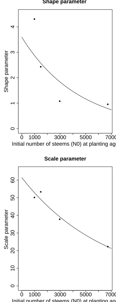
The parameter estimates,γ_k andβ_k,k= 1,3,4,5, are displayed in Figure 3, plotted against the correspond-ing plantcorrespond-ing densities (in stems per ha). Also shown are exponential functions that were fitted to these points. This relationship is potentially useful in that it allows one, by means of interpolation, to estimate the param-eters of the lifetime distribution for planting densities that are different from those that were investigated in the experiment. In a second estimation pass we there-fore estimated these two exponential functions directly from the original data by maximizing a single combined likelihood function. Since the resulting curves did not change much, we will not give details of the second, and more complicated, computation here.

Having estimated the survival distribution as a func-tion ofN0 we are now in a position to estimate the dis-tribution of the number of trees that are survive any given aget. Given that there areN0 trees initially, the number of trees that survive to agetcan be regarded as a binomial experiment withN0 trails. Each trial results in one of two mutually exclusive outcomes, survival and death. The Weibull distribution is used to estimate the binomial parameter, namely the probability that a tree survives longer thanttime units, sayp_t(also called the ‘probability of success’). The number of surviving trees ttime units after planting is binomially distributed ran-dom variable with parametersN0andpt= 1−F(t; γ, β) where γ and β can be estimated the exponential func-tion displayed in Figure 3 from the known value N0. The probability that precisely nof theN0 trees survive longer thanttime units is given by

N0

n

pn_t(1−p_t)N0−n_{, n= 0,1, . . . N}

0. (8)

0 1000 3000 5000 7000

01234

Shape parameter

Initial number of steems (N0) at planting age

Shape par

ameter

0 1000 3000 5000 7000

0

1

02

03

04

05

06

0

Scale parameter

Initial number of steems (N0) at planting age

Scale par

ameter

Figure 3: Weibull shape and scale parameters estimated from the number of trees per ha planted.

Thus (and, for simplicity, dropping the subscript k) N_i, i = 1,2, . . . ,8 is binomially distributed with first parameter (the number of trials) equal to N0 and sec-ond parameter (the probability of success) is given by 1−F(A_i; γ, β).

tri-als is N_i−1, and the probability of success is given by 1−F(A_i;γ, β)/(1−F(A_i−1;γ, β)). This probability is computed using a left-truncated Weibull distribution so as to take account of the fact that the N_i−1 trees have already survivedA_i−1 time units after planting.

2.2.3 Unconditional distribution stand basal area Models (3)-(5), which are based on the ‘alterna-tive approach’, contain the covariate N_i, the concur-rent number of surviving trees. These models only de-scribe the conditional distribution of log(G_i) for given values of N_i. We will assume that these conditional distributions are normal and have a constant variance.

Theunconditionaldistribution of log(G_i) is then a

mix-ture distribution; its density is a weighted sum of

condi-tional (normal) densities taken over all possible values of N_i. The weights are given by the binomial probabilities P(N_i = n). Thus the density of log(G_i), which is not itself normal, is given by:

N0

n=0

P(N_i=n)·

φ(E(log(G_i)|N_i =n, N_i−1, Gi−1, Ai−1, Ai), σ2),

where φ(μ, σ2_{) represents the density of a normal} dis-tribution with mean μ and varianceσ2_{. Although the} range ofN_i extends from 0 toN0, we will omit the term with n=0 in the above sum in order to avoid taking the log of zero when computing the unconditional dis-tributions. This is reasonable ifA_i is not ‘too large’ or, more precisely, ifA_iis such that the probability thatall

N0 trees will die withinAi years after planting is small enough to be negligible.

The main motivation for considering Models (3)-(5) is to take account of tree survival in the modeling of basal area, because, as is illustrated in Figure 1, the rate of survival in unthinned forests can vary enormously as a function of planting density. One can take survival into account by includingN_i as a covariate in the model for basal area. However, having done this, one must then also account for the variability in the distribution of basal area that is attributable to uncertainties regard-ing how many trees will survive. This can be done by computing the unconditional distribution of the (log) basal area. We note that this is not the same as simply replacing the term N_i in the conditional distribution of log(G_i) by E(N_i), because the distribution of log(G_i) is different to that of log(G_i|N_i = E(N_i)). The latter is a normal distribution, whereas the former is a mix-ture of normals. The mixmix-ture distribution has following moments (Fr¨uhwirth-Schnatter, 2006):

Expectation:

E(log(G_i)) =μ ≈

N0

n=1

P(N_i=j)μ_n (9)

Variance:

E(log(G_i)−μ)2) ≈ N0

n=1

P(N_i=n)(μ_n2+σ2_n)−μ2 (10)

whereμ_n denotes the mean, andσ2_n the variance, of the conditional distribution of log(G_i|N_i=n). We assume that all the conditional variances are equal. The above moments are approximations because we have omitted the summand forn= 0.

2.2.4 Model evaluation criteria Three different model selection criteria were applied for comparing the models that describe the log of stand basal area growth. The Bayesian Information Criterion: BIC = −2 log(L(ˆθ)) + log(n)d, where log(L(ˆθ)) represents the estimated maximum log-likelihood of the model, n the sample size anddthe number of estimated parameters. This affords a balance between the quality of the fit, which is measured by the log-likelihood term, and com-plexity, as measured by the ‘penalty term’ log(n)d. The model with the smallest BIC is judged best. Akaike’s Information Criterion,AIC =−2 log(L(ˆθ)) + 2d), has a similar structure but uses a different penalty term. Ex-cept for very small samples the BIC applies a more severe penalty for complexity than does the AIC. For a discus-sion of these criteria see, e.g., Zucchini (2000). We also report values of the residual standard error: RSE=√σˆ2_, where ˆσ2=

i(Yi−Yi)2

degrees of freedom is the estimated residual variance. In terms of this criterion the model for which RSE is the minimum should be selected (Maddala and Lahiri, 2009).

3

Results

In this section we present the parameter estimates and the results for the models for tree survival and basal area growth that were outlined in the previous section.

which gives a total of 32 data points. The estimated exponential function of the shape parameter,γ, and the scale parameter,β, of the Weibull distribution are given by the following functions of N0 (measured in units of stems per ha):

γ= 3.5927 exp(−0.000225N0) (11)

β = 61.4138 exp(−0.000152N0) (12) These relationships make it possible to estimate the parameters of the Weibull distribution function for arbi-trary planting density in the range 0 to 7000 stems per ha (see Figure 3). The estimated Weibull parameters for each plot of the dataset are shown in Table 2. The Weibull distribution functions for Plots 1,3,4,5 are dis-played in Figure 4. It can be seen that the probability that a tree dying in the very dense Plot 1, is initially much greater than in the other, less dense, plots. As expected, the probability of tree survival increases with decreasing number of trees per unit area. Although the distribution functions in Figure 4 are displayed for the age range 0 to 120 years, it has to be kept in mind that the observation interval covered less 40 years. Conse-quently, the available data do not provide information about the lifetime distribution of trees that are older than 40 years; the extrapolations beyond that age are based on the assumption that the Weibull model con-tinues to hold beyond 40 years. Since this assumption cannot be checked with the available data, the said ex-trapolations obviously need to be regarded as hopeful approximations.

Table 2: Weibull Parameter estimated for each plot from equations (11) and (12).

Plot 1 Plot 3 Plot 4 Plot 5

Shape 0.79 1.84 2.57 2.88

Scale 22.14 39.17 49.04 52.87

3.2 Basal area growth The parameters of all mod-els were estimated using linear least squares techniques available in the software environment R. For model es-timation successive interval data, all starting from the age at planting, were used.

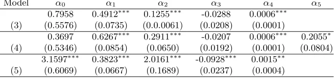
Table 3 gives the parameters estimates, standard er-rors, the values of the selection criteria for Models (1) and (2). Table 4 gives a summary of the results Models (3) to (5), all of which use the number of surviving trees as covariate.

The results clearly indicate that the models which use the number of surviving trees as covariate, i.e. Mod-els (3)-(5), lead to much better fits than do those that

t

distr

ib

ution function

Plot= 1

Plot= 3

Plot= 4

Plot= 5

0 20 40 60 80 100 120

0.0

0.2

0.4

0.6

0.8

1.0

Figure 4: Graph of the cumulative Weibull distribution functions for different initial stem numbers at planting.

do not, namely Models (1) and (2). All three model selection criteria, given in Tables 3 and 5, are substan-tially lower for the models in the first group. Within the group (3)-(5), Model (3) is judged worst by all three criteria. The RSE of Model (4) and (5) are very similar and Model(5) has the lowest AIC and BIC values. Since Model (5) is also the simplest of the three it is the model used in the following section.

Table 5: Values of the model selection criteria for Models (3) - (5).

Model RSE AIC BIC

(3) 0.180 -12.29 -3.50 (4) 0.164 -17.47 -7.21 (5) 0.165 -17.91 -9.12

distribu-Table 3: Results for Models (1) and (2): the estimated parameter values and goodness-of-fit statistics.

Model (1), Schumacher (1939) Model (2), Rodr´ıguez-Soalleiro (1995)

ˆ

α1= 3.0979 (Std. Error 0.2417)∗∗∗ α0ˆ =−0.7470 (Std. Error 0.7020)

ˆ

α1= 1.1993 (Std. Error 0.5525)∗

ˆ

α2=−1.3565 (Std. Error 0.6001)∗

RSE = 0.6727 RSE = 1.076

AIC = 68.42 BIC = 71.35 AIC = 82.41 BIC = 88.28

Stat. significant:∗∗∗ at 0,1% level,∗∗ at 1% level,∗at 5% level,·at 10% level

Table 4: Estimated parameters model (3), model (4) and model (5).

Model α0 α1 α2 α3 α4 α5

0.7958 0.4912∗∗∗ 0.1255∗∗∗ -0.0288 0.0006∗∗∗

(3) (0.5576) (0.0735) (0.0.0061) (0.0208) (0.0001)

0.3697 0.6267∗∗∗ 0.2911∗∗∗ -0.0207 0.0006∗∗∗ 0.2055∗

(4) (0.5346) (0.0854) (0.0650) (0.0192) (0.0001) (0.0804)

3.1597∗∗∗ 0.3823∗∗∗ 2.0161∗∗∗ -0.0928∗∗∗ 0.0015∗∗

(5) (0.6069) (0.0667) (0.1689) (0.0237) (0.0004)

Values of standard errors given in parenthesis.

Stat. significant: ∗∗∗at 0,1% level,∗∗ at 1% level,∗at 5% level,·at 10% level

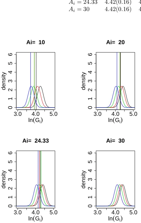
tion for the respective age; none of the realizations fall in an extreme tail. Note that there are no horizontal lines for the case A_i = 30. That is because no observation was made at that age. This illustrates the point that, despite the fact that the number of trees that were alive 30 years after planting is unknown, it is possible never-theless to estimate the distribution of the log basal area for stands of that age using Model (5). Table 6 presents the expected values and the standard deviations of the fitted unconditional distributions for the ages covered in Figure 5.

We remark on some features of the estimated prop-erties of the unconditional distributions, some of which are given in Table 6.

• The variance remains nearly constant with increas-ing age. It seems to be independent of the plantincreas-ing density.

• As might be expected, each different planting den-sity leads to a different unconditional distribution for basal area and the differences are substantial in the first few years. Somewhat surprising is that these differences seem to persist. Our estimates in-dicate that, if convergence to a single distribution occurs, then it takes longer than 40 years before the effects of planting density become small.

• The estimated mean log basal area for Plots 1 and 3, which have the higher planting densities, increases

over the first 20 years and then remains approx-imately constant, whereas it increased monotoni-cally in Plots 4 and 5. Presumably this is conse-quence of higher tree mortality, combined with a reduced diameter growth rate in Plots 1 and 3.

4

Discussion

esti-Table 6: Expected values and standard deviation (in brackets) of the estimated unconditional distribution of log(Stand Basal Area) for four different ages and four different planting densities. Note that no data were available for ageA_i = 30.

Plot 1 Plot 3 Plot4 Plot5

A_i= 10 4.28(0.15) 4.14(0.15) 3.90(0.15) 3.75(0.15) A_i= 20 4.44(0.16) 4.37(0.15) 4.17(0.15) 4.03(0.15) A_i= 24.33 4.42(0.16) 4.36(0.15) 4.19(0.15) 4.06(0.15) A_i= 30 4.42(0.16) 4.36(0.16) 4.22(0.16) 4.10(0.16)

3.0 4.0 5.0

0123456

Ai= 10

ln

(

)

density

3.0 4.0 5.0

0123456

Ai= 20

ln

(

)

density

3.0 4.0 5.0

0123456

Ai= 24.33

ln

(

)

density

3.0 4.0 5.0

0123456

Ai= 30

ln

(

)

density

Figure 5: Unconditional distributions Black: Plot 1, red: Plot 3, green: Plot 4, blue: Plot 5 Vertical line: observed values atA_i.

mate the unconditional distribution of the log basal area for any planting density within a specified range.

The Langsaeter hypothesis (Langsaeter, 1944) states that the total volume production in a stand of a given age, composition and site is, for all practical purposes, constant for a wide range of density of stocking. The results of this study do not support this hypothesis (see Gilmore et al., 2005 and Zeide, 2004). The distribu-tion of the future basal area in an unthinnedEucalyptus

grandisforest on the Zululand coastal plain is not

inde-pendent of the planting density, within the (rather wide) range of the experimental densities investigated in this study. The results presented here provide clear evidence that planting density has strong and long-lasting effects on basal area. Our estimates indicate that these effects persist for at least 40 years and that, even after length of time, the rate of convergence is very slow.

Acknowledgment

We are grateful to the two anonymous referees for their numerous and very helpful comments and sugges-tions.

References

´

Alvarez-Gonz´alez, J.G. and R. Rodr´ıguez-Soalleiro and G. Vega Alonso. 1999. Elaboraci´on de un modelo de crecimiento din´amico para rodales regulares de Pinus pinaster Ait. en Galicia. Investigaci´on Agraria: Sis-temas y Recursos Forestales 8: 319–334.

Amateis, R.L. and P.J. Radtke and H.E. Burkhart. 1995. TAUYIELD: a stand-level growth and yield model for thinned and unthinned loblolly pine plantations. School of Forestry and Wildlife Resources. VPI and SU. Report No. 82.

Belisle, C.J.P. 1992. Convergence theorem for a class of simulated annealing algorithms on Rd_{. Journal of} Applied Probabilty. 29(4): 885–895.

Bredenkamp, B.V. 1984. The CCT concept in spacing research - a review. P. 313–332 in Proc. of the IUFRO Symposium on site and productivity of fast growing plantations, Grey, D.C., A.P.G. Sch”onau, C.J. Schutz (eds.). South Africa Forestry Research Institute.

Burgers, T.F. 1976. Management graphs derived from the correlated (CCT) projects: South Africa. For. Res. Inst. Bull. 54. Dept. Forestry. Pretoria. South Africa. 60 p.

Burkhart, H.E. 2003. Suggestions for choosing an ap-propriate level for modelling forest stands. P. 3–10 in Modelling Forest Systems, Amaro, A., D. Reed, P. Soares (eds.). CAB International. Oxfordshire. UK.

Castedo-Dorado, F. and U. Di´eguez-Aranda and J.G. ´

Alvarez Gonz´alez. 2007. A growth model for Pinus radiata D. Don stands in north-western Spain. Annals of Forest Science 64: 453–465.

Cieszewski C.J. and M. Harrison and S.W. Martin. 2000. Practical methods for estimating non-biased parame-ters in self-referencing growth and yield models. Uni-versity of Georgia. PMRC Tech. Rep. 2000-7. 10 p.

Clutter J.L. and E.P. Jones E.P. 1980. Prediction of growth after thinning in oldfield slash pine planta-tions. USDA For. Serv. Pap. 217. 14 p.

Cox, D.R. and D. Oakes. 1984. Analysis of Survival Data. Chapman & Hall. London.

Craib, I.J. 1939. Thinning, Pruning and management studies on the main exotic conifers grown in South Africa. Dept. of Agric. and For. Bull. 196. Govt. Printer. Pretoria. 179 p.

Decourt, N. 1974. Remarque sur une rela-tion dendrom´etrique inattendue-cons´equences m´ethodologiques pour la construction des tables de production. Annales des Sciences Foresti´eres 31: 47–55.

Di´eguez-Aranda, U. and F. Castedo and J.G. ´ Alvarez-Gonz´alez and A. Rojo. 2006. Dynamic growth model for Scots pine (Pinus sylvestris L.) plantations in Gali-cia (north-western Spain). Ecological Modelling 191: 225–242.

Fr¨uhwirt-Schnatter, S. 2006. Finite Mixture and Markov Switching Models. Springer. New York.

Gadow, K.v. 1987. Untersuchungen zur Konstruktion von Wuchsmodellen f¨ur schnellw¨uchsige Plantagen-baumarten. Forstl. Forschungsberichte 77. Universit¨at M¨unchen. 147 p.

Gadow, K.v. and B.V. Bredenkamp. 1992. Forest Man-agement. Academica Press. Pretoria.

Gadow, K.v. 1996. Modelling growth in managed forests - realism and limits of lumping. The Science of the Total Environment 183: 167–177.

Garc´ıa, O. 1988. Growth modelling — a (re)view. New Zealand Journal of Forestry Science 33 (3): 14–17.

Garc´ıa, O. 1994. The State-Space Approach in Growth Modeling. Canadian Journal of Forest Research-Revue Canadienne de Recherche Forestiere 24: 1894– 1903.

Garc´ıa, O. 2003. Dimensionality reduction in growth models: an example. Forest biometry, Modelling and Information Sciences 1: 1–15.

Gilmore D.W. and T.C. O’Brien and H.M. Hogan-son. 2005. Thinning Red Pine Plantations and the Langsaeter Hypothesis: A Northern Minnesota Case Study. Northern Journal of Applied Forestry 22(1): 19–26.

Ihaka, R. and R. Gentleman. 1996. R: a language for data analysis and graphics. Journal of Computational and Graphical Statistics 5(3): 299–314.

Langsaeter, A. 1944. Om tynning i enaldret gran-og fu-ruskog. Medd. Det norske Skogforsoksvesen 8: 131– 216.

Maddala, G.S. and K. Lahiri. 2009. Introduction to Econometrics. 4th Ed. Wiley. Chichester.

Marsh, E.K. 1957. Some preliminary results from O’Connor’s correlated curve trend (CCT) experiments on thinning and espacements and their practical sig-nificance. 7th British Commonwealth forestry confer-ence. Government Printer. 52 p.

Matyssek, R. 2003. Kosten und Nutzen von Raumbeset-zung und -ausbeute. AFZ/Der Wald 17: 862–863.

Milsum, J.H. 1966. Biological Control Systems Analysis. McGraw–Hill. New York.

O’Connor, A.J. 1935. Forest research with special refer-ence to planting distances and thinning. Brit. Emp. For. Conf. 30 p.

O’Connor, A.J. 1960. Thinning research. J. of the South African For. Assoc. 34: 65–88.

Pienaar, L.V. and K.J. Turnbull. 1973. The Chapman-Richards generalization of von Bertalanffy’s growth model for basal area growth and yield in evenaged stands. Forest Science 19(1): 2–22.

Schumacher, F. X. 1939. A new growth curve and its application to timber yield studies. J. of Forestry 37: 819–820.

Vanclay, J.K. 1995. Growth models for tropical forests: a synthesis of models and methods. Forest Science 41: 7–42.

Van Laar, A. 1982. The response o f Pinus radiata to initial spacing. South African For. J. 121: 52–63.

Zeide, B. 2004. Optimal stand density: a solution. Cana-dian Journal of Forest Research 34(4): 846–854.