www.theoryofcomputing.org
Distribution-Free Testing Lower Bounds for
Basic Boolean Functions
Dana Glasner
∗Rocco A. Servedio
†Received: September 18, 2008; published: October 17, 2009.
Abstract: In thedistribution-freeproperty testing model, the distance between functions is measured with respect to an arbitrary and unknown probability distributionDover the input domain. We consider distribution-free testing of several basic Boolean function classes over {0,1}n, namely monotone conjunctions, general conjunctions, decision lists, and linear
threshold functions. We prove that for each of these function classes, Ω((n/logn)1/5) oracle calls are required for any distribution-free testing algorithm. Since each of these function classes is known to be distribution-free properly learnable (and hence testable) usingΘ(n)oracle calls, our lower bounds are polynomially related to the best possible.
ACM Classification:F.2.2, G.3
AMS Classification:68Q99, 68W20
Key words and phrases: property testing, distribution-free testing, decision list, conjunction, linear threshold function
1
Introduction
The field of property testing deals with algorithms that decide whether an input object is in a certain class or is far from being in the class after reading only a small fraction of the object. Property testing was formally introduced in [22] after significant prior work [5,4] and has evolved into a rich field of study (see [3,8,11,20,21] for some surveys). A standard approach in property testing is to view the input to the testing algorithm as a function over some finite domain; the testing algorithm is required to distinguish functions that are in a certain classC from functions that areε-far from being in class
∗Supported in part by an FFSEAS Presidential Fellowship.
C. In the most commonly considered property testing scenario, a function f is ε-far from class Cif
f disagrees with every functiong that is in classC on at least anε fraction of the points in the input
domain; equivalently, the distance between functions f andgis measured with respect to the uniform distribution over the domain. The testing algorithm “reads” f by adaptively querying a black-box oracle for f at points x of the algorithm’s choosing (such oracle calls are often referred to as “membership queries” in computational learning theory). The main goal in designing property testing algorithms is to use as few queries as possible to distinguish the two types of functions; ideally the number of queries should depend only onε and should be independent of the size of f’s domain.
In recent years there has been considerable work in the standard “uniform distribution” property testing scenario on testing various natural Boolean function classes. Some classes for which uniform distribution testing results have been obtained are monotone functions [7, 10, 12]; Boolean literals, monotone conjunctions, general conjunctions ands-term monotone DNFs [19];J-juntas [9]; parity func-tions (which are equivalent to degree-1 polynomials) [5]; degree-dpolynomials [2]; decision lists,s-term DNFs, size-sdecision trees ands-sparse polynomials [6]; and linear threshold functions [18].
Distribution-free property testing A natural generalization of the notion of property testing is to consider a broader notion of the distance between functions. Given a probability distributionDover the domain, we may define the distance between f andgas the probability that an inputxdrawn from D satisfies f(x)6=g(x); the “standard” notion of property testing described above corresponds to the case whereDis the uniform distribution. Distribution-free property testing is the study of property testers in a setting where distance is measured with respect to afixed but unknown and arbitraryprobability distributionD. Since the distributionDis unknown, in this scenario the testing algorithm is allowed to draw random samples fromDin addition to querying a black-box oracle for the value of the function.
Distribution-free property testing is well-motivated by very similar models in computational learning theory (namely the model of distribution-free PAC learning with membership queries, which is closely related to the well-studied model of exact learning from equivalence and membership queries), and by the fact that in various settings the uniform distribution may not be the best way to measure distances. Distribution-free property testing has been considered by several authors [1,13,16,14,15]; we briefly describe some of the most relevant prior work below.
Goldreich et al.[13] introduced the model of distribution-free property testing, and observed that anyproperdistribution-free PAC learning algorithm (a learning algorithm for a class of functions that always outputs a hypothesis function that itself belongs to the class) can be used to directly obtain a distribution-free property testing algorithm. They also showed that several graph properties that have testing algorithms with query complexity independent of input size in the uniform-distribution model (such as bipartiteness,k-colorability,ρ-clique,ρ-cut andρ-bisection) do not have distribution-free
test-ing algorithms with query complexity independent of input size. In contrast, Halevy and Kushilevitz [14] gave a distribution-free algorithm for testing connectivity in sparse graphs that has poly(1/ε)query
com-plexity independent of input size.
A range of positive and negative results have been established for distribution-free testing of Boolean functions over{0,1}n. Halevy and Kushilevitz [15] showed that any distribution-free monotonicity
test-ing algorithm over{0,1}n must make 2Ω(n) queries; this is in contrast with the uniform distribution
10,12]. On the other hand, [16] showed that for several important function classes over{0,1}nsuch
as juntas, parities, low-degree polynomials and Boolean literals, there exist distribution-free testing al-gorithms with query complexity poly(1/ε)independent of n; these distribution-free results match the
query bounds of uniform distribution testing algorithms for these classes.
To sum up, the current landscape of distribution-free property testing is intriguingly varied. For some testing problems (juntas, parities, Boolean literals, low-degree polynomials, connectivity in sparse graphs) the complexity of distribution-free testing is known to be essentially the same as the complexity of uniform-distribution testing; but for other natural testing problems (monotonicity, bipartiteness,k -colorability,ρ-clique,ρ-cut,ρ-bisection), distribution-free testing provably requires many more queries than uniform-distribution testing.
This work Our work is motivated by the fact that for many Boolean function classes over{0,1}nthat
are of fundamental interest, a very large gap exists between the query complexities of the best known distribution-free property testing algorithms (which typically follow trivially from learning algorithms and have query complexityΩ(n)) and the best known uniform distribution property testing algorithms (which typically have query complexity poly(1/ε) independent ofn). A natural goal is to try to close
this gap, either by developing efficient distribution-free testing algorithms or by proving lower bounds for distribution-free testing for these classes.
We study distribution-free testability of several fundamental classes of Boolean functions that have been previously considered in the uniform distribution testing framework, and have been extensively studied in various distribution-free learning models. More precisely, we consider the following classes (in order of increasing generality): monotone conjunctions, arbitrary conjunctions, decision lists, and linear threshold functions. Each of these four classes is known to be testable in the uniform distribution setting using poly(1/ε)queries, independent ofn(see [19] for monotone and general conjunctions, [6] for decision lists, and [18] for linear threshold functions). On the other hand, for each of these classes the most efficient known distribution-free testing algorithm is simply to use a proper learning algorithm. Using the fact that each of these classes has Vapnik-Chervonenkis dimension Θ(n), standard results in learning theory yield well-known algorithms that useO(n/ε)random examples and no membership
queries (see, e. g., Chapter 3 of [17]), and known results also imply that any learning algorithm must makeΩ(n)oracle calls (see [23]).
Our main results are strong distribution-free lower bounds for testing each of these four function classes. As our first main result, we prove:
Theorem 1.1. Let T be any algorithm which, given oracle access to an unknown function f :{0,1}n→
{0,1} and (sampling) oracle access to an unknown distribution Dover {0,1}n, outputs “yes” with probability at least2/3if f is a monotone conjunction, and outputs “no” with probability at least2/3if f is1/6-far from every decision list with respect toD. Then T must makeΩ((n/logn)1/5)oracle calls
in total.
Since every monotone conjunction and conjunction can be expressed as a decision list, we have the following corollary:
Additionally, for the case of linear threshold functions we have:
Theorem 1.3. Let T be any algorithm which, given oracle access to an unknown function f :{0,1}n→
{0,1} and (sampling) oracle access to an unknown distribution Dover {0,1}n, tests whether f is a linear threshold function or is1/4-far from every linear threshold function with respect toD. Then T must makeΩ((n/logn)1/5)oracle calls in total.
These results show that for these function classes, distribution-free testing is nearly as difficult (from a query perspective) as distribution-free learning, and is much more difficult than uniform-distribution testing. We remind the reader that unlike several models of learning, testing is not monotone with respect to inclusion: in other words, ifC0 is a subclass ofC, an efficient algorithm for testingCdoes not immediately imply an efficient algorithm for testingC0. As an example of this, the empty class consisting of no functions is trivially testable, and the “complete” class consisting of all functions is also trivially testable, but many intermediate classes are not trivially testable.
Our Approach For simplicity, we discuss here only the construction for the lower bound for monotone conjunctions. The basic idea is to construct two distributionsYESandNOover pairs(h,D)whereh
is a Boolean function andDis a distribution over the boolean cube such that for every pair(g,Dg)in the support ofYES, the functiongis a monotone conjunction and for every pair(f,Df)in the support of NO, the function f is far from every monotone conjunction with respect to the distribution Df.
We then show that any algorithm that makes fewer thanΩ((n/logn)1/5) queries can only distinguish between a draw from theYES-distribution and theNO-distribution with probability at most 1/4. Since a distribution-free tester must distinguish between the two with probability at least 2/3, this implies that any distribution-free tester must make at leastΩ((n/logn)1/5)queries.
For both theYESandNOdistributions, a draw from the distribution is obtained by first randomly choosingmtriples ofn-bit strings (a1,b1,c1), . . . ,(am,bm,cm). The 2mstringsa1,b1,a2,b2, . . . ,am,bm
each have (disjoint) sets of`bits set to 0 andn−`bits set to 1; each stringci is the bitwise-and ofai
andbi. (See the description of distributionHinSection 3.1.1for a more detailed description.) A draw of(g,Dg)fromYESis constructed in such a way thatg(ai) =0,g(bi) =1 andg(ci) =0 for eachi; the distributionDgputs weight 2/(3m)on eachbi point and weight 1/(3m)on eachci point. We defineg
over the rest of the points in the boolean cube so thatgis a monotone conjunction. (SeeSection 3.1.2
for details.)
In contrast, a draw of(f,Df)fromNOis constructed such that f(ai) =1, f(bi) =1 but f(ci) =0, and the distributionDf puts 1/(3m)weight on eachai, bi,orci point. (See Section 3.1.3for details.) As noted in [19], any monotone conjunctionhmust satisfyh(x)∧h(y) =h(x∧y)(wherex∧ydenotes the bitwise AND ofxandy) for allx,y∈ {0,1}n, and so no monotone conjunctionhcan satisfyh(ai) = h(bi) =1 buth(ci) =0. Thus, every monotone conjunction must differ from f on at least one ofai,bi,
ci, for each of themtriples, and f is at least 1/3-far from every monotone conjunction.
The bulk of our work is to additionally show that queries “do not help” the tester. While there are various technical complications that need to be dealt with in the formal proof, the high-level idea is that an algorithm can only distinguish between a draw from theYES-distribution andNO-distribution if it manages to query certain types of points called “witnesses” (seeSection 3.3). We show that witnesses are very hard to find when allowed onlyo((n/logn)1/5)queries since intuitively, a witness can only be found by random guessing (see the proof ofLemma 3.11).
Organization After giving preliminaries in Section 2, in Section 3 we present our construction of “yes” and “no” (function, distribution) pairs that are used in the lower bound for monotone conjunctions, conjunctions and decision lists as well as the proof of the lower bound. InSection 4we describe a variant of the construction for linear threshold functions, and use it to prove the lower bound for linear threshold functions.
2
Preliminaries
Throughout the paper we deal with Boolean functions overninput variables.
Definition 2.1.LetDbe a probability distribution over{0,1}n. Given Boolean functions f,g:{0,1}n→
{0,1}, thedistance between f and g with respect toDis defined by distD(f,g) =Prx∼D[f(x)6=g(x)].
IfCis a class of Boolean functions over{0,1}n, we define thedistance between f and C with respect toDto be distD(f,C) =ming∈CdistD(f,g).
We say that f isε-far from C with respect toDif distD(f,C)≥ε.
Now we can define the notion of a distribution-free tester for a class of functionsC:
Definition 2.2. Adistribution-free tester for class Cis a probabilistic oracle machineT which takes as input a distance parameterε>0 and is given access to
• a black-box oracleto a fixed (but unknown and arbitrary) function h:{0,1}n → {0,1} (when
invoked with inputx, the oracle returns the valueh(x)); and
• asampling oraclefor a fixed (but unknown and arbitrary) distributionDover{0,1}n(each time
it is invoked this oracle returns a pair(x,h(x))wherexis independently drawn fromD).
T must satisfy the following two conditions: for anyh:{0,1}n→ {0,1}and any distributionD,
• ifhbelongs toC, then Pr[Th,D=Accept]≥2 3; and
• ifhisε-far fromCw.r.t. D, then Pr[Th,D=Accept]≤13.
Notation and Terminology For a stringx∈ {0,1}n we writex
i to denote theith bit ofx. Forx,y∈
{0,1}nwe writex∧yto denote then-bit stringzwhich is the bitwise AND ofxandy, i. e.,zi=xi∧yi
for alli. The stringx∨yis defined similarly to be the bitwise OR ofxandy.
Recall that thetotal variation distance, orstatistical distance, between two random variablesX and
Y that take values in a finite setSis
dTV(X,Y) =
1 2
∑
ζ∈S
|Pr[X=ζ]−Pr[Y =ζ]|.
The classes we consider For completeness we define here all the classes of functions that we will consider: these are (in order of increasing generality) monotone conjunctions, general conjunctions, decision lists, and linear threshold functions. We note that each of these function classes is quite basic and natural and has been studied intensively in fields such as computational learning theory.
Definition 2.3. The class MCONJ consists of all monotone conjunctions of any subset of Boolean variables fromx1, . . . ,xn, i. e., all ANDs of (unnegated) Boolean variables.
Definition 2.4. The class CONJ consists of all conjunctions of any subset of Boolean literals over{0,1}n
(a literal is a Boolean variable or the negation of a variable).
Definition 2.5. Adecision list Lof lengthkover the Boolean variablesx1, . . . ,xnis defined by a list ofk pairs and a bit(`1,β1),(`2,β2), . . . ,(`k,βk),βk+1where each`i is a Boolean literal and eachβi is either
0 or 1. Given anyx∈ {0,1}n,the value ofL(x)is
βiifiis the smallest index such that`iis made true by x; if no`iis true thenL(x) =βk+1. Let DL denote the class of all decision lists of arbitrary lengthk≥0 over{0,1}n.
Definition 2.6. Alinear threshold function is defined by a list ofn+1 real valuesw1, . . . ,wn,θ. The
value of the function on inputx∈ {0,1}nis 1 ifw
1x1+· · ·+wnxn≥θand is 0 ifw1x1+· · ·+wnxn<θ. We write LTF to denote the class of all linear threshold functions over{0,1}n.
It is well known and easy to see that MCONJ(CONJ(DL(LTF.
3
The lower bound for monotone conjunctions
In this section we will prove the following theorem:
Theorem 3.1. Let q= (1/20)(n/logn)1/5. There exist two distributions,YESandNO, over pairs(h,D)
where h:{0,1}n→ {0,1}is a Boolean function andDis a distribution over the domain{0,1}n that have the following properties:
1. For every pair(g,Dg)in the support ofYES, the function g is a monotone conjunction.
Moreover, for any probabilistic oracle algorithm T that, given a pair(h,D), makes at most q black-box queries to h and samplesDat most q times, we have
Pr
(g,Dg)∼YES
[Tg,Dg =Accept]− Pr
(f,Df)∼NO
[Tf,Df =Accept]
≤1 4.
Note that in the above theorem each probability is taken over the draw of the (function,distribution) pair from the appropriate distributionYESorNO, over the random draws from the distributionDf or
Dg, and over any internal randomness of algorithmT.
A simple corollary ofTheorem 3.1gives us our main result:
Corollary 3.2. Distribution-free testing of monotone conjunctions, conjunctions, and decision lists all requireΩ(n/logn)1/5queries.
Proof. Since MCONJ⊂CONJ⊂DL, properties (1) and (2) imply that any distribution-free tester for MCONJ,CONJ or DL that is run with distance parameterε =1/6 must accept a random pair(g,Dg)
drawn fromYES with probability at least 2/3, and must accept a random pair (f,Df) drawn from NOwith probability at most 1/3. Therefore, byTheorem 3.1, any such tester must make at leastq=
Ω(n/logn)1/5queries.
3.1 The two distributions
We now define the two distributions,YESandNO, and prove that these distributions have properties (1) and (2) required byTheorem 3.1. Our constructions are parameterized by three values`,mands. As we will see the optimal setting (up to multiplicative constants) of these parameters for our purposes is
`=n2/5(logn)3/5, m= (n/logn)2/5, s=logn. (3.1)
To keep the different roles of these parameters clear in our exposition we will present our constructions and analyses in terms of “`,” “m,” and “s” as much as possible and only plug in the values from (3.1) toward the end of our analysis.
We first define the distributionHover tuples
(R,A1,B1, . . . ,Am,Bm,α1, . . . ,αm),
whereA1,B1, . . . ,Am,Bmare disjoint`-element subsets of[n], the setRequalsSi(Ai∪Bi), andαi is an
element ofAifor eachi. It is useful to define this distribution since a draw from both theYESandNO distributions begins with a draw fromH.
3.1.1 TheHdistribution
A draw from the distributionHover(R,A1,B1, . . . ,Am,Bm,α1, . . . ,αm)tuples is obtained as follows:
• For eachi=1, . . . ,mletα(i)be an element chosen uniformly at random from the setAi; we say
thatα(i)is arepresentativeofAi.
Given a draw(R,A1,B1, . . . ,Am,Bm,α1, . . . ,αm)fromH, we define the stringsa1,b1,c1, . . . ,am,bm, cmin the following way: Letai∈ {0,1}nbe the string whose jthbit is 0 iffj∈Ai. The stringbiis defined
similarly. The stringci is defined to beai∧bi. Similarly we define the setCi=Ai∪Bi. We sometimes
refer toai,bi,cias the “points of theith block.”
Additionally, we define the conjunctiong1to be the conjunction of all variables in[n]\R.
3.1.2 The YES distribution
A draw from the distributionYESover(g,Dg)pairs is obtained as follows:
• Make a draw from theHdistribution to obtain(R,A1,B1, . . . ,Am,Bm,α1, . . . ,αm).
• The distributionDgputs weight 2/(3m)onbiand puts weight 1/(3m)oncifor eachi=1, . . . ,m.
• Define the function g2 as follows: g2 is a conjunction of length m formed by taking g2(x) =
xα(1)∧ · · · ∧xα(m), i. e.,g2is an AND of the representatives from each ofA1, . . . ,Am.
• The functiongis defined as:g=g1∧g2.
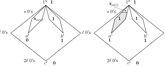
It is clear that for every(g,Dg)in the support ofYES, the functiongis a monotone conjunction that contains exactlyn−2`m+mvariables, so Property (1) ofTheorem 3.1indeed holds. We also note that for eachiwe haveg(ai) =g(ci) =0 andg(bi) =1; see Figure 1.
1
1n
s0’s
xα(i) 1
ℓ0’s
ai bi
1 0
2ℓ0’s ci 0
000000000 000000000 000000000 000000000 000000000 000000000 000000000 000000000 000000000 000000000 000000000 000000000
111111111 111111111 111111111 111111111 111111111 111111111 111111111 111111111 111111111 111111111 111111111 111111111
1
1n
s0’s xα(i)
1 1
ℓ0’s
ai bi
1 1
2ℓ0’s ci 0
Figure 1: The left figure shows how a yes-functionglabelsci and the points above it (includingai and
bi). Bold print indicate the label thatg assigns. Note that every point abovebi is labeled1 byg, and
points aboveaiare labeled according toxααα(i). The right figure shows how a no-function f labelsci and
3.1.3 The NO distribution
A draw from the distributionNOof(f,Df)pairs is obtained as follows:
• Make a draw from theHdistribution to obtain(R,A1,B1, . . . ,Am,Bm,α1, . . . ,αm).
• The distributionDf is uniform over the 3mpointsa1, . . . ,cm.
• Define the function f0as follows: f0(x) =0 if there exists somei∈[m]such that both the following conditions hold:
– xα(i)=0 and
– {fewer thansof the elements j∈Aihavexj=0)}or{xj=0 for some j∈Bi}.
• The final function f is defined as f=g1∧f0.
SeeFigure 1for a pictorial representation of the yes-functiongand the no-function f. With the definition ofNOin place, we now establish Property (2) ofTheorem 3.1:
Lemma 3.3. For any pair(f,Df)in the support ofNOand any decision list h, the function f is at least
1/6-far from h w.r.t.Df.
Proof. Fix any(f,Df)in the support ofNOand any decision list
h= (`1,β1),(`2,β2), . . . ,(`k,βk),βk+1.
We will show that at least one of the six points a1,b1,c1,a2,b2,c2 is labeled differently byh and f. Grouping allmblocks into pairs and applying the same argument to each pair gives the lemma.
Let first(a1) be the index of the first literal, `first(a1), in h that is satisfied by the point a1, so the
valueh(a1)equalsβfirst(a1). Define first(b1),first(c1), first(a2), first(b2), and first(c2)similarly. We will
assume thathand f agree on all six points, i. e., thatβfirst(a1)=βfirst(b1)=βfirst(a2)=βfirst(b2)=1 and
βfirst(c1)=βfirst(c2)=0, and derive a contradiction.
We may suppose w.l.o.g. that first(a1) =min{first(a1),first(b1),first(a2),first(b2)}. We now con-sider two cases depending on whether or not first(c1)<first(a1). (Note that first(a1) cannot equal first(c1)since f(a1) =1 but f(c1) =0.)
Suppose first that first(c1)<first(a1). No matter what literal`first(c1)is, sincec1 satisfies`first(c1)at
least one ofa1,b1must satisfy it as well. But this means that min{first(a1),first(b1)} ≤first(c1), which is impossible since first(c1)<first(a1)and first(a1)≤min{first(a1),first(b1)}.
Now suppose that first(a1) <first(c1); then it must be the case that `first(a1) is a literal “xj” for
some j∈B1. (The only other possibilities are that `first(a1)is “xj” for some j∈Ai or is “xj” for some j∈([n]\C1); in either case, this would imply that f(c1) =1, which does not hold.) Since f(c2) =0 and(c2)j=1, it must be the case that first(c2)<first(a1). But no matter what literal`first(c2)is, sincec2
satisfies it at least one ofa2andb2must satisfy it as well. This means that
min{first(a2),first(b2)} ≤first(c2)<first(a1)≤min{first(a2),first(b2)},
In fact, we have a slightly stronger result for the case of testing monotone conjunctions. For any
(f,Df) drawn fromNO, we have f(ai) = f(bi) =1 and f(ci) =0 for each i=1, . . . ,m. It is noted
in [19] (and is easy to check) that any monotone conjunctionhmust satisfy h(x)∧h(y) =h(x∧y)for allx,y∈ {0,1}n, and thus must satisfyh(ci) =h(ai)∧h(bi). Thus any monotone conjunctionh must
disagree with f on at least one ofai,bi,ci for alli, and consequently f is 1/3-far from any monotone conjunction with respect toDf.
Thus we have established properties (1) and (2) stated at the beginning of this section.
3.2 The idea
In this subsection we attempt to explain the main ideas of the proof ofTheorem 3.1. Before we give the main ideas we first provide some preliminary intuition and useful terminology.
It is easy to see that in both the yes-case (when the (function, distribution) pair is drawn fromYES) and the no-case (when the (function, distribution) pair is drawn fromNO), any black-box query that sets any variable in[n]\Rto 0 will get a 0 response. To give some preliminary intuition for our construction, let us explain here the role that the large conjunctiong1(overn−2`mvariables) plays in both theYES andNOcases. The idea is that because ofg1, a testing algorithm that has obtained stringsz1, . . . ,zqfrom the distributionDwill “gain nothing” by querying any stringxthat has any bitxi set to 0 that was set to 1 in all ofz1, . . . ,zq. This is because such a variablexiwill with very high probability (over a random
choice of(f,Df)fromNOor a random choice of(g,Dg)fromYES) be contained in[n]\R, so in both the “yes” and “no” cases the query will yield an answer of 0 with very high probability. Consequently there is no point in making such a query in the first place. (We give a rigorous version of this argument inSection 3.3.2.)
The following terminology will be useful: we say that an inputx∈ {0,1}n isi-special if (at least selements j∈Ai havexj=0) and (xj=1 for all j∈Bi). Thus an equivalent way to define f0 is that f0(x) =g2(x)unlessg2(x) =0 (because somexα(i)=0) andxisi-special for eachisuch thatxα(i)=0;
in this case f0(x) =1.
Here is some high-level intuition for the proof. IfT could findai,biandcifor someithenT would know which case it is in (yes versus no), becauseh(ai)∧h(bi) =h(ci)if and only ifT is in the yes-case. SinceT can only makeq√mdraws fromD, the birthday paradox tells us that with high probability the random sample thatT draws contains at most one ofai,biandcifor eachi. Theci-type points (with
n−2`ones) are labeled negative in both the yes- and no- cases, so these “look the same” toT in both cases. Other than theci-type points, in the yes-case the distributionsDg put weight only on thebi-type points (withn−`ones) which are positively labeled, and in the no-case the distributionsDf put weight only on theai- andbi-type points (withn−`ones) which are also positively labeled. So the draws with
n−`ones “look the same” toT as well in both cases. So with high probabilityT cannot distinguish between yes-pairs and no-pairs on the basis of the firstqrandom draws alone. (Corollary 3.5formalizes this intuition.)
Consider a single fixed blocki∈[m]. If none ofai,bi orciare drawn in the initial sample, then by the argument at the start of this subsection, the tester will get no useful information about which case it is in from this block. By the birthday paradox we can assume that at most one ofai,biandciis drawn in the initial sample; we consider the three cases in turn.
Ifbiis drawn, then again by the argument at the start of this subsection all query points will have all the bits inAi set to 1; such queries will “look the same” in both the yes- and no- cases as far as theith
block is concerned.
Ifaiis drawn (so we are in the no-case), then by the same argument all query points will have all the bits inBiset to 1. Using the definition of f0, as far as theith block is concerned with high probability it will “look like” the initialai point was abi-point from the yes-case. This is because the only way the tester can tell that it is in the no-case is if it manages to query a point which has fewer thansbits from
Ai set to 0, but the representativeα(i)is one of those bits. Such points are hard to find sinceα(i) is randomly selected fromAi. (See the “a-witness” case in the proof ofLemma 3.11.)
Finally, suppose thatci is drawn. The only way a tester can distinguish between the yes- and no-cases is by finding ani-special point (or determining that no such point exists), but to find such a point it must make a query with at leasts0’s inCi, all of which lie inAi. This is hard to do since the tester
does not know how the elements ofCi are divided into the setsAi andBi. (See the “c-witness” case in the proof ofLemma 3.11.)
3.3 Proof ofTheorem 3.1
Fix any probabilistic oracle algorithmT that makes at most q black-box queries to h and samplesD at mostq times. Without loss of generality we may assume that T first makes exactly qdraws from distributionD, and then makes exactlyq(adaptive) queries to the black-box oracle forh.
It will be convenient for us to assume that algorithm T is actually given “extra information” on certain draws from the distributionD. More precisely, we suppose that each timeT calls the oracle for
D,
• If a “ci-type” labeled example(ci,h(ci))is generated by the oracle, algorithmT receives the triple
(ci,h(ci),α(i))(recall thatα(i)is the index of the variable fromCithat belongs to the conjunction g2);
• If a “non-ci-type” labeled example (x,h(x))is generated by the oracle wherex6=ci for all i=
1, . . . ,m, algorithmT receives the triple(x,h(x),0). (Thus there is no “extra information” given on non-cipoints.)
It is clear that provingTheorem 3.1 for an arbitrary algorithmT that receives this extra information establishes the original theorem as stated (for algorithms that do not receive the extra information).
Following [15], we now define aknowledge sequenceto precisely capture the notion of “what an algorithm learns from its queries.” A knowledge sequence is a sequence of elements corresponding to the interactions that an algorithm has with each of the two oracles. The firstqelements of a knowledge sequence are triples as described above; each corresponds to an independent draw from the distribution
algorithm’s calls to the black-box oracle forh. (Recall that these later oracle calls are adaptive, i. e., each query point can depend on the answers received from previous oracle calls.)
Notation For any oracle algorithmALG,let PALGyes denote the distribution over knowledge sequences
induced by runningALGon a pair(g,Dg)randomly drawn fromYES. Similarly, letPALGno denote the
distribution over knowledge sequences induced by runningALGon a pair(f,Df)randomly drawn from NO. Where there is no risk of confusion we will sometimes write PALGyes to denote a random variable
drawn from this distribution, and similarly forPALGno .
For 0≤i≤qwe writePALGyes,ito denote the length-(q+i)prefix of a knowledge sequence drawn from
PALG
yes , and similarly forPALGno,i.
We will proveTheorem 3.1by showing that the statistical distancedTV(PT
yes,PTno)between
distribu-tionsPTyesandPTnois at most 1/4.
3.3.1 Most sequences of draws are “clean” in both the yes- and no- cases
The main result of this subsection isCorollary 3.5; intuitively, this corollary shows that given onlyq
draws from the distribution and no black-box queries, it is impossible to distinguish between the yes-and no- cases with high accuracy. This is achieved via the notion of a “clean” sequence of draws from the distribution, which we now explain.
LetS=x1, . . . ,xq be a sequence of qexamples drawn from distribution D, whereDis eitherDf
for some(f,Df)∼NOorDg for some(g,Dg)∼YES. In either case there is a corresponding set of pointsa1,b1,c1, . . . ,am,bm,cm as described in Section 3.1, corresponding to the initial draw from the
Hdistribution. We say thatSiscleanifSdoes not hit any block 1, . . . ,mtwice, i. e., if the number of different blocks fromi=1, . . . ,mfor whichScontains some pointai,biorciis exactlyq.
We note that strictly speaking, cleanliness is not a property of a sequenceSdrawn fromDf orDg, but rather a property of the way the sequenceSis generated (since it depends on the random choice of
ai,bi,ci, i. e., on the draw fromH). With this understood, for conciseness we shall speak of cleanliness simply as a property of a sequenceSof draws fromDf orDg. We further note that while a draw from
PT
no,0is, strictly speaking, a sequence ofqtriples (as described at the beginning ofSection 3.3), without risk of confusion we will simply write “S∼PT
no,0” to indicate the corresponding sequence of draws from
Df (and likewise we write “S∼PT
yes,0” to indicate the corresponding sequence of draws fromDg). With this notion and these conventions in place, we have the following claim and its easy corollary:
Claim 3.4. We have
Pr
S∼PT yes,0
[S is clean] = Pr
S∼PT no,0
[S is clean]≥1−q2/m.
Furthermore, the conditional random variables
(S|S is clean)S∼PT
yes,0 and (S|S is clean)S∼PTno,0
Proof. We first show that
Pr
S∼PT yes,0
[Sis clean] = Pr
S∼PT no,0
[Sis clean]≥1−q2/m.
Actually, we will prove something stronger, which is that regardless of which(g,Dg) is drawn from
YES, the conditional probability of getting a clean sequence is at least 1−q2/m. Fix any(g,Dg) in the support ofYES, and consider the outcomes ofS∼PT
yes,0corresponding to this(g,Dg)being drawn fromYES. Since each independent draw fromDg hits each block 1, . . . ,mwith probability 1/m, the probability thatS∼PT
yes,0is clean is
q
∏
i=1
1−i−1
m
≥1−q2/m.
The same argument shows that PrS∼PT
no,0[Sis clean]also equals∏ q i=1 1−
i−1
m
.
Now we show that the conditional random variables are identically distributed. It is not difficult to see that for any 0≤ j≤q−1, given any particular length-jprefix of a draw fromPTyes,0, conditioned on the draw fromPTyes,0being clean, the(j+1)-st element of the draw fromPTyes,0has
• a 2/3 chance of being a triple(x,1,0)where x∈ {0,1}n has `zeros and the locations of the `
zeros are selected uniformly at random (without replacement) from the set of those bit positions that had value 1 in all jof the previous draws;
• a 1/3 chance of being a triple (x,0,α) where x has 2` zeros, the locations of the 2`zeros are
selected uniformly at random (without replacement) from the same set of bit positions described above, andα is an index drawn uniformly at random from the indices of the 2`zeros inx.
It is also not difficult to see that given any particular length-jprefix of a draw fromPTno,0, conditioned on the draw fromPTno,0 being clean, the(j+1)-st element of the draw fromPTno,0 is distributed in the exact same way.
Corollary 3.5. The statistical distance dTV(PT
yes,0,PTno,0)is at most q2/m.
Proof. We can express the statistical distance betweenPT
yes,0andPTno,0as
1 2
∑
ζPrS∼PT
yes,0[(S=ζ)&(Sis clean)] +S∼PrPT yes,0
[(S=ζ)&(Snot clean)]
− Pr
S∼PT no,0
[(S=ζ)&(Sis clean)]− Pr
S∼PT no,0
[(S=ζ)&(Snot clean)]
.
By parts (1) and (2) of the claim, we have that
Pr
S∼PT yes,0
[(S=ζ)&(Sis clean)] = Pr
S∼PT no,0
for allζ. Thus we can reexpress the statistical distance as 1 2
∑
ζ PrS∼PT yes,0
[(S=ζ)&(Snot clean)]− Pr
S∼PT no,0
[(S=ζ)&(Snot clean)]
.
This is at most
1 2
Pr
S∼PT yes,0
[Snot clean] + Pr
S∼PT no,0
[Snot clean]
which is at mostq2/mby part (1) of the claim.
3.3.2 Eliminating foolhardy queries
LetT1denote a modified version of algorithmT which works as follows: likeT, it starts out by making
qdraws from the distribution. LetQbe the set of all indicesisuch that allqdraws from the distribution have theith bit set to 1. We note that for both the yes-distribution and the no-distribution, we have that
[n]\Ris contained inQ. Moreover, ifi∈[m]is such that none of{ai,bi,ci}occur among theqdraws, thenCi is also contained inQ.
We say that any query stringx∈ {0,1}nthat hasx
j=0 for some j∈Qisfoolhardy. After making
itsq draws from D, algorithmT1 simulates algorithmT for q black-box queries, except that for any foolhardy query thatT makes,T1 “fakes” the query in the following sense: it does not actually make the query but instead proceeds asT would proceed if it made the query and received the response 0.
Our goal in this subsection is to show that in both the yes- and no- cases, the executions ofT andT1
are statistically close. (Intuitively, this means that we can w.l.o.g. assume that the testing algorithmT
does not make any foolhardy queries.) To analyze algorithmT1it will be useful to consider some other algorithms that are intermediate betweenT andT1, which we now describe.
For each value 1≤k≤q, letUkdenote the algorithm which works as follows:Ukfirst makesqdraws from the distributionD, then simulates algorithmT forkqueries, except that for each of the firstk−1 queries thatT makes, if the query is foolhardy thenUk “fakes” the query as described above. LetUk0
denote the algorithm which works exactly likeUk, except that if thekthquery made byUkis foolhardy thenUk0 fakes that query as well. We have the following:
Lemma 3.6. For all k∈[q], the statistical distance
dTV (PUk
yes|P Uk
yes,0is clean),(P
Uk0 yes|P
Uk0
yes,0is clean)
is at most2`m/n, and similarly
dTV (PUnok |P Uk
no,0is clean),(P
Uk0 no|P
Uk0
no,0is clean)
is also at most2`m/n.
The executions ofUk andUk0are identically distributed unless thekthquery string (which we denote z) is foolhardy and the black-box functionghasg(z) =1. Consequently the variation distance
dTV (PUk
yes|P Uk
yes,0is clean),(P
Uk0 yes|P
Uk0
yes,0is clean)
is at most
Pr[(zis foolhardy)&(g(z) =1)]≤Pr[(g(z) =1)|(zis foolhardy)],
where the probabilities are taken over a random draw of(g,Dg)fromYESconditioned on(g,Dg)being consistent with theqdraws from the distribution and with the firstk−1 queries, and with theqdraws from the distribution being clean.
Since the firstk−1 queries do not involve any variables inQ(because foolhardy queries are faked for the firstk−1 queries) and our analysis will only concern variables inQ, to analyze this conditional probability it is enough to consider(g,Dg)drawn fromYESconditioned on (g,Dg)being consistent with theq draws from the distribution and with theseqdraws being clean. Suppose that these draws from the distribution yieldrdistinctci-type points (each with 2`zeros) and(q−r)distinctbi-type points (each with`zeros). Then after these draws, the algorithm “knows”(r+q)`elements ofR. LetZdenote the set of these(r+q)`elements ofR. The setRalso contains 2`m−(r+q)`other “unknown” variables from among the|Q|=n−(r+q)`variables in[n]\Z.
We would like to find the probability, over random (g,Dg) drawn from YESconsistent with the draws from the distribution, thatg(z) =1 given thatz is foolhardy. Sincez is foolhardy there must be at least one index j∈[n]\Z such thatzj=0. So the desired probability is at most the probability that j belongs to R, since if j∈/ Rthe conjunction g1 will evaluate to 0 onz. For a random (g,Dg) that is consistent with the draws from the distribution, the remaining 2`m−(r+q)`elements ofR\Z are chosen randomly from then−(r+q)`elements of[n]\Z. Consequently the probability that jbelongs toR\Zis
2`m−(r+q)` n−(r+q)` ≤
2`m n ,
and the lemma is proved.
Now a hybrid argument usingLemma 3.6lets us bound the statistical distance between the execu-tions ofT andT1.
Lemma 3.7. The statistical distance dTV(PT1
yes,PTyes) is at most2`mq/n+q2/m, and the same bound holds for dTV(PT1
no,PTno).
Proof. We prove the yes-case; the no-case follows by an identical argument. ByClaim 3.4, at the cost ofq2/mindTV(PT
1
yes,PTyes)we may assume that the draws from the
distribu-tion are clean. So we henceforth in the proof always condidistribu-tion on the draws from the distribudistribu-tion being clean, and we will bounddTV(PT1
yes,PTyes)by 2`mq/nunder this conditioning on each argument todTV.
We use induction onito show thatdTV(PTyes,i,P T1
yes,i)is at most 2`mi/nfor alli. Once we have this,
takingi=qand recalling thatPTyes,q=PTyesandPT 1
yes,q=PT 1
yesgives the desired bound.
For the induction step we assume thatdTV(PTyes,i,P T1
yes,i)≤2`mi/n, and we will show that
dTV(PTyes,i+1,PyesT1,i+1)≤2`m(i+1)
n .
We first note that the random variablesPT1
yes,i+1 and P
Ui0+1
yes are identically distributed, i. e., they have
statistical distance zero.Lemma 3.6now implies thatdTV(PT 1 yes,i+1,P
Ui+1
yes )is at most 2`m/n. Since
dTV(PTyes1,i+1,PTyes,i+1)≤dTV(PTyes1,i+1,PUi+1
yes ) +dTV(P Ui+1 yes ,P
T yes,i+1),
it is enough to bounddTV(PUi+1
yes ,PTyes,i+1)by 2`mi/n. But since the firstq+ielements of the sequence
PUi+1
yes are distributed according toPT 1
i (and the last element is obtained by performing the(i+1)-st query
ofT), we have that dTV(PUi+1
yes ,PTyes,i+1) =dTV(PT 1
yes,i,PTyes,i), and by the induction hypothesis this is at
most 2`mi/n. This concludes the proof.
3.3.3 Bounding the probability of finding a witness
LetT2 denote an algorithm that is a variant of T1, modified as follows. T2 simulates T1 except that
T2does not actually make queries on non-foolhardy strings. InsteadT2simulates the answers to those queries “in the obvious way” that they should be answered if the target function were a yes-function and hence all of the draws fromDthat yielded strings with`zeros were in factbi-type points. More precisely, assume that there arer distinctci-type points in the initial sequence ofq draws from the distribution. Since for eachci-type point the algorithm is givenα(i), the algorithm “knows”rvariablesxα(i)that are
in the conjunction. The algorithmT2 simulates an answer to a non-foolhardy queryx∈ {0,1}n with 0
if any of ther xα(i)variables are set to 0 inx, and with 1 otherwise. Note that consequentlyT2does not
actually make any black-box queries at all.
In this subsection we will show that in both the yes- and no- cases, the executions of T1 and T2
are statistically close; once we have this it is not difficult to complete the proof ofTheorem 3.1. In the yes-case these distributions are in fact identical (Lemma 3.8), but in the no-case these distributions are not identical; we will argue that they are close using properties of the function f0fromSection 3.1.3.
We first address the easier yes-case:
Lemma 3.8. The statistical distance dTV(PT 1 yes,PT
2
yes)is zero.
Proof. We argue for every query, the two algorithmsT1 andT2receive (or simulate) the same answer. Fix any 1≤i≤qand letzdenote theithquery made byT.
Ifzis a foolhardy query then bothT1andT2 simulate an answer of 0. So suppose that zis not a foolhardy query. Then any 0’s thatz contains must be in positions from points that were sampled in the first stage. Consequently the only variables that can be set to 0 that are in the conjunctiongare the
xα(i)variables from theCi sets corresponding to theci points in the draws. All the other variables that
were assigned value 0 in some string that was drawn from the distribution are not in the conjunction, so setting them to 0 or 1 will not affect the value ofg(z). Therefore, the valueg(z)thatT1receives in response to the query stringzis 0 if any of thexα(i)variables are set to 0 inz, and is 1 otherwise. This is
To handle the case, we introduce the notion of a “witness” that the black-box function is a no-function.
Definition 3.9. We say that a knowledge sequence contains awitnessfor(f,Df)if elementsq+1,q+
2, . . .of the sequence (i. e., the black-box queries) contain either of the following:
1. A pointz∈ {0,1}nsuch that for some 1≤i≤mfor whichaiwas sampled in the firstqdraws, the
bit zα(i) is 0 and fewer thansof the elements j∈Ai havezj =0. We refer to such a point as an a-witness for block i.
2. A pointz∈ {0,1}nsuch that for some 1≤i≤mfor whichci was sampled in the firstqdraws,z
isi-special. We refer to such a point as ac-witness for block i.
The following lemma implies that it is enough to bound the probability thatPTnocontains a witness:
Lemma 3.10. The statistical distance
dTV (PT 1 no |PT
1
no does not contain a witness andPT 1
no,0is clean),
(PTno2 |PTno2 does not contain a witness andPTno2,0is clean)
is zero.
Proof. Claim 3.4 implies that(PTno1,0 | PT1
no,0 is clean) and (PT
2 no,0 | PT
2
no,0 is clean) are identically dis-tributed. We show that if there is no witness, then for every query the algorithmsT1andT2receive (or simulate) the same answer as each other; this gives the lemma. Fix any 1≤i≤qand letzdenote theith
query.
Ifzis a foolhardy query, then bothT1andT2 simulate an answer tozwith 0. So suppose thatz is not a foolhardy query and not a witness. Then any 0’s thatzcontains must be in positions from points that were sampled in the first stage.
First suppose that one of thexα(i)variables from someci that was sampled is set to 0 inz. Sincezis
not a witness, eitherzhas fewer thanszeros fromAior some variable fromBiis set to 0 inz. So in this case we have f(z) =g2(z) =0.
Now suppose that none of thexα(i)variables from theci’s that were sampled are set to 0 inz. If no
variablexα(i)from anyai that was sampled is set to 0 inz, then clearly f(z) =g(z) =1. If any variable
xα(i) from anai that was sampled is set to 0 in z, then sincez is not a witness there must be at leasts
elements ofAiset to 0 and every element ofBiset to 1 for each suchxα(i). Therefore, f(z) =1.
Thus the value f(z) thatT1 receives on queryz is 0 if any of thexσ(i) variables from theci’s that were sampled is set to 0 inz, and the value f(z)is 1 otherwise. This is exactly how T2 simulates its answer to the queryzas well.
k−1 queries is faked (foolhardy queries are faked as described in the previous subsection, and non-foolhardy queries are faked as described at the start of this subsection). Thus algorithmVk actually makes at most one query to the black-box oracle, thekth one (if this is a foolhardy query then this one is faked as well). LetVk0 denote the algorithm which works exactly likeVk, except that if thekth query
made byVkis non-foolhardy thenVk0 fakes that query as well as described at the start of this subsection.
Lemma 3.11. For each value1≤k≤q, the statistical distance
dTV (PVk
no|P Vk
no,0is clean),(P
Vk0 no|P
Vk0
no,0is clean)
is at mostmax{qs`,2qs}. (This equals
qs
` provided that s2
s≥`, as is the case in our parameter settings
given by(3.1).)
Proof. ByLemma 3.10, the executions ofVkandVk0are identically distributed unless thekthquery string (which we denotez) is a witness for(f,Df). Since neitherVknorVk0makes any black-box query prior to z, the variation distance betweenPVk
noandP Vk0
nois at most Pr[zis a witness], where the probability is taken
over a random draw of(f,Df)fromNOconditioned on(f,Df)being consistent with theqdraws from the distribution and with those firstqdraws being clean. We bound the probability thatzis a witness by considering both possibilities forz(ana-witness or ac-witness) in turn.
• We first bound the probability thatzis ana-witness. So fix somei∈[m]and let us suppose that
ai was sampled in the first stage of the algorithm. We will bound the probability thatzis an a -witness for blocki; once we have done this, a union bound over the (at mostq) blocks such that
aiis sampled in the first stage gives a bound on the overall probability thatzis ana-witness.
Fix any possible outcome for z. In order for z to be an a-witness for block i, it must be the case that fewer thans of the`elements inAi are set to 0 inz, but the bitzα(i) is set to 0. For a
random choice of(f,Df)as described above, since we are conditioning on theqdraws from the distribution being clean, the only information that theseqdraws reveal about the indexα(i)is that it is some member of the setAi. Consequently for a random(f,Df)as described above, each bit inAi is equally likely to be chosen asα(i), so the probability thatα(i)is chosen to be one of the
at most sbits inAi that are set to 0 inz is at mosts/`. Consequently the probability thatzis an
a-witness for blockiis at mosts/`,and a union bound gives that the overall probability thatzis ana-witness is at mostqs/`.
• Now we bound the probability thatz is ac-witness. Fix somei∈[m]and let us suppose thatci
was sampled in the first stage of the algorithm. We will bound the probability thatzis ac-witness for blockiand then use a union bound as above.
Fix any possible outcome forz; letrdenote the number of 0’s thatzhas in the bit positions inCi. In order forzto be ac-witness for blockiit must be the case thatzisi-special, i. e.,r≥sand allr
of these 0’s in fact belong toAi. For a random choice of(f,Df)conditioned on being consistent with the q samples from the distribution and with thoseq samples being clean, the distribution over possible choices ofAiis uniform over all 2``
Consequently the probability that allr0’s belong toAiis at most
2`−r
`−r
2` `
=
`(`−1)· · ·(`−r+1)
2`(2`−1)· · ·(2`−r+1)<
1 2r ≤
1 2s.
So the probability thatzis ac-witness for blockiis at most 1/2s, and by a union bound the overall
probability thatzis ac-witness is at mostq/2s.
So the overall probability that z is a witness is at most max{qs`,2qs}. Using (3.1) we have that the
maximum isqs/`, and the lemma is proved.
Now similar to Section 3.3.2, a hybrid argument using Lemma 3.11lets us bound the statistical distance between the executions ofT1andT2. The proof of the following lemma is entirely similar to that ofLemma 3.7so we omit it.
Lemma 3.12. The statistical distance dTV(PT1 no,PT
2
no)is at most q2s/`+q2/m.
3.3.4 Putting the pieces together
At this stage, we have thatT2 is an algorithm that only makes draws from the distribution and makes no queries. It follows that the statistical distancedTV(PT
2 yes,PT
2
no)is at mostdTV(PTyes,0,P
T
no,0). So we can bounddTV(PTyes,PTno)as follows (we write “d” in place of “dTV” for brevity):
dTV(PTyes,PnoT ) ≤ d(PTyes,PTyes1) +d(PTyes1,PTyes2) +d(PTyes2,PnoT2) +d(PTno2,PTno1) +d(PTno1,PTno)
≤ d(PTyes,PT 1
yes) +d(PT 1 yes,PT
2
yes) +d(PTyes,0,PTno,0) +d(PT
2 no,PT
1
no) +d(PT 1 no,PTno)
≤ 4q2/m+4q`m/n+q2s/`
where the final bound follows by combiningCorollary 3.5,Lemma 3.7,Lemma 3.8andLemma 3.12. Recalling the parameter settings`=n2/5(logn)3/5,m= (n/logn)2/5,ands=lognfrom (3.1) and the fact thatq= (1/20)(n/logn)1/5, this bound is less than 1/4. This concludes the proof ofTheorem 3.1.
4
A lower bound for linear threshold functions
The basic approach is similar to that ofSection 3, and indeed several ingredients from the earlier proof can be directly reused; we focus our discussion on the points where the approaches differ. We shall prove the following:
Theorem 4.1. Let q= (1/20)(n/logn)1/5. There exist two distributions,YESandNO, over pairs(h,D)
where h:{0,1}n→ {0,1}is a Boolean function andDis a distribution over the domain{0,1}n that have the following properties:
1. For every pair(g,Dg)in the support ofYES, the function g is a linear threshold function.
Moreover, for any probabilistic oracle algorithm T that, given a pair(h,D), makes at most q black-box queries to h and samplesDat most q times, we have
Pr
(g,Dg)∼YES
[Tg,Dg =Accept]− Pr
(f,Df)∼NO
[Tf,Df =Accept]
≤1 4.
Since any distribution-free tester for LTF that is run with distance parameterε=1/4 must accept a random pair(g,Dg) drawn fromYESwith probability at least 2/3, and must accept a random pair
(f,Df)drawn fromNOwith probability at most 1/3, we have the following corollary ofTheorem 4.1,
which gives us our main result:
Corollary 4.2. Distribution-free testing of linear threshold functions requiresΩ(lognn)1/5queries.
4.1 The two distributions for linear threshold functions
The construction fromSection 3is not suited for a lower bound on LTF (observe that for any(f,Df)in
the support ofNOthe function f is 0-far from the linear threshold functionx1+· · ·+· · ·xn≥n−3`/2 with respect toDf), so we need a different approach.
In the rest of this section we define two distributionsYESandNOover pairs(h,D)and prove that these distributions have properties (1) and (2) described inTheorem 4.1.
InSection 4.2we use these distributions to prove a lower bound for LTF.
Before giving the precise construction, here is a very rough first intuition for how it works. Recall that in the earlier construction, we relied on the fact that no monotone conjunctionhcan satisfyh(1,0) =
h(0,1) =1 buth(0,0) =0. For linear threshold functions, we will instead rely on the fact that no linear threshold function can satisfyh(0,0) =h(1,1) =0 buth(1,0) =h(0,1) =1.
4.1.1 The YES distribution
As in Section 3 our constructions are parameterized by values `, m and s that are set according to Equation (3.1) inSection 3. A draw from the distributionYESover(g,Dg)pairs is obtained as follows:
• As before, make a draw from theHdistribution to obtain(R,A1,B1, . . . ,Am,Bm,α1, . . . ,αm).
• The distributionDgputs 1/4 weight on the point 1n, and puts weight 1/(2m)onbiand 1/(4m)on
cifor alli=1, . . . ,m.
• The functiongis defined as follows:
g(x) =1 if and only if all three of the following conditions hold:
1. xj=1 for all j∈([n]\R);
2. xj=1 for all j=α(1), . . . ,α(m); and
It is straightforward to show that an equivalent way to define g is as follows: g(x) equals 1 if
u(x)≥θand equals 0 ifu(x)<θ, where
u(x) = 10n2
∑
j∈([n]\R)xj+5n m
∑
i=1
xα(i)− m
∑
i=1k∈Ci,
∑
k6=α(i)xk, (4.1)
θ = 10n2(n−2`m) +5nm−m(2`−1) +s. (4.2)
Fix any(g,Dg)in the support ofYES. It is clear thatgis a linear threshold function. It is straight-forward to check that
u(1n) =10n2(n−2`m) +5nm−m(2`−1),
u(ci) =10n2(n−2`m) +5n(m−1)−(m−1)(2`−1),and
u(bi) =10n2(n−2`m) +5nm−m(2`−1) +` ,
and consequently we haveg(1n) =g(ci) =0,g(bi) =1.
4.1.2 The NO distribution
A draw from the distributionNOof(f,Df)pairs is obtained as follows:
• As in the yes-case, make a draw from theHdistribution to obtain
(R,A1,B1, . . . ,Am,Bm,α1, . . . ,αm).
• The distributionDf puts weight 1/4 on 1n, puts 1/4 weight uniformly over thempointsc1, . . . ,cm, and puts 1/2 weight uniformly over the 2mpointsa1,b1, . . . ,am,bm.
• The function f is defined as follows. Given inputx, letJ(x)⊆[m]be the set of thoseisuch that
xisi-special as defined inSection 3.2(i. e., theith block ofxhas no zeros inBi but has at leasts
zeros inAi.)
f(x) =1 if and only if all three of the following conditions hold:
1. xj=1 for all j∈([n]\R);
2. For allisuch thatxisnot i-special,xα(i)=1; and
3. |J(x)|(`−1) +∑i∈J(x)∑k∈Aixk+∑i∈([m]\J(x))∑k∈Ci,k6=α(i)xk≤m(2`−1)−s.
It is straightforward to show that an equivalent way to define f is as follows: f(x) equals 1 if
v(x)≥θand equals 0 ifv(x)<θ. Hereθis defined as in (4.2) andv(x)is defined as follows:
v(x) = 10n2
∑
j∈([n]\R)xj+5n |J(x)|+
∑
i∈([m]\J(x))xα(i) !
−|J(x)|(`−1)−
∑
i∈J(x)
∑
k∈Ai
xk−
∑
i∈([m]\J(x))
∑
k∈Ci,k6=α(i)
Here is some intuition for the definition of f. Suppose that testing algorithmT manages to query an input stringxwhich hasxj =1 for all j∈Bi but also has at leastsbits inAi set to 0. Then as we will
see, it must be the case that the algorithm actually drew the pointaiin its sample fromDf. So in order forT to be “fooled” into thinking that the function is aYESfunction, we want the contribution from the bits ofAi andBi for this input to “look like” the function is aYESfunction for which the pointai that was drawn fromDf is actually a pointbi drawn fromDg. This is the rationale behind the definition of
f; instead of computingu(x)and comparing it withθ, we computev(x), which reverses the role ofAi
andBibits on those blocks.
It is easy to see that in both the yes-case and the no-case, any black-box query that sets any variable in[n]\Rto 0 will give a 0 response. As in the earlier construction, intuitively this will let us assume that any testing algorithm that has obtained stringsz1, . . . ,zqfrom the distributionDnever queries any string
xthat has any bitxiset to 0 that was set to 1 in all ofz1, . . . ,zq.
Finally, it is easy to check that for any(f,Df)drawn fromNO, we have
v(1n) =10n2(n−2`m) +5nm−m(2`−1),
v(ci) =10n2(n−2`m) +5n(m−1)−(m−1)(2`−1),and
v(ai) =v(bi) =10n2(n−2`m) +5nm−m(2`−1) +` .
(Note that these values on 1n,ciandbiare the same that the corresponding functionsu(x)would take in the yes-case.) Thus we have f(1n) =f(ci) =0 and f(ai) = f(bi) =1 for eachi=1, . . . ,m. It is easy to see that any linear threshold function must disagree with f on at least one of the four points 1n,ai,bi,ci
for eachi. Consequently f is at least 1/4-far from any linear threshold function with respect toDf. Thus we have established Properties (1) and (2) as stated inTheorem 4.1.
4.2 Proof ofTheorem 4.1
As inSection 3.3, letT be any fixed oracle algorithm that makes exactlyqdraws from the distribution and then makes exactlyq black-box queries. All notation such asPTno,0 and the like is defined anal-ogously to the definitions given inSection 3.3. We again assume thatT is given “extra information” as described earlier when it draws ci-type examples from the distribution (so the testing algorithm is assumed to actually receive triples instead of pairs, as inSection 3.3). Our definition of a knowledge sequence and of a “clean” sequence of draws are the same as before.
The following easy claim is an analogue ofClaim 3.4:
Claim 4.3. We havePr[PTyes,0is clean] =Pr[PTno,0 is clean]≥1−q2/m. Furthermore, the conditional random variables(PT
yes,0|PTyes,0is clean)and(PTno,0|PTno,0is clean)are identically distributed.
Proof. We first show that Pr[PTyes,0is clean] =Pr[PTno,0is clean]≥1−q2/m. Fix any(g,Dg)in the sup-port ofYES, and consider the outcomes ofPT
yes,0corresponding to this(g,Dg)being drawn fromYES. Since each independent draw fromDg hits each block 1, . . . ,mwith probability 3/4m, the probability thatPTyes,0is clean is
q
∏
i=1
1−3(i−1) 4m
≥1−3q 2
The same argument shows that Pr[PT
no,0is clean]also equals∏
q i=1
1−3(4i−m1).
Now we show that the conditional random variables are identically distributed. It is not difficult to see that for any 0≤ j≤q−1, given any particular length-jprefix ofPTyes,0, conditioned onPTyes,0being clean, the(j+1)-st element ofPT
yes,0has
• a 1/4 chance of being the triple(1n,0,0);
• a 1/2 chance of being a triple(x,1,0)where x∈ {0,1}n has `zeros and the locations of the `
zeros are selected uniformly at random (without replacement) from the set of those bit positions that had value 1 in all jof the previous draws;
• a 1/4 chance of being a triple (x,0,α) where x has 2` zeros, the locations of the 2`zeros are
selected uniformly at random (without replacement) from the same set of bit positions described above, andα is an index drawn uniformly at random from the indices of the 2`zeros inx.
It is also not difficult to see that given any particular length-jprefix ofPTno,0, conditioned onPTno,0being clean, the(j+1)-st element ofPT
no,0is distributed in the exact same way. This proves the lemma.
The proof of the following corollary is identical to the proof ofCorollary 3.5:
Corollary 4.4. The statistical distance dTV(PTyes,0,P
T
no,0)is at most q2/m.
Foolhardy queries can be handled just as before. Let the algorithms T1, Uk andUk0 be defined
precisely as inSection 3.3.2. The arguments ofSubsection 3.3.2immediately yield:
Lemma 4.5. For all k∈[q], the statistical distance
dTV (PUk
yes|P Uk
yes,0is clean),(P
Uk0 yes|P
Uk0
yes,0is clean)
is at most2`m/n, and similarly dTV (PUk
no|P Uk
no,0is clean),(P
Uk0 no|P
Uk0
no,0is clean)
is also at most2`m/n.
Lemma 4.6. The statistical distance dTV(PT 1
yes,PTyes) is at most2`mq/n+q2/m, and the same bound holds for dTV(PT
1 no,PTno).
As we now describe, the details of how non-foolhardy queries are handled are different from Sec-tion 3.3.3.
LetT2denote an algorithm that is a variant ofT1, modified as follows. T2simulatesT1except that
T2does not actually make queries on non-foolhardy strings; insteadT2simulates the answers to those queries “in the obvious way” that they should be answered if the target function were a yes-function and hence all of the draws fromDthat yielded strings with`zeros were in factbi-type points. More precisely, assume that there arer distinctci-type points in the initial sequence ofq draws from the distribution. Since for eachci-type point the algorithm is givenα(i), the algorithm “knows”r variablesxα(i). The
algorithmT2simulates an answer to a non-foolhardy queryz∈ {0,1}nas follows:T2computes
u0(z) =10n2(n−2`m) +5n(m− |I0|)−m(2`−1) +|K\I0|
• Kis the set of all variablesxiset to 0 inz, and
• I0is the set of “known”xα(i)variables that are set to 0 inz
and answers 1 ifu0(z)≥θ, and answers 0 otherwise.
Lemma 4.7. The statistical distance dTV(PTyes1,PT 2
yes)is zero.
Proof. We argue thatT1andT2answer all queries in exactly the same way. Fix any 1≤i≤qand letz
denote theithquery made byT.
Ifzis a foolhardy query then bothT1andT2answerzwith 0. So suppose thatzis not a foolhardy query. By inspection of (4.1), we can reexpressu(z)as
u(z) =10n2(n−2`m) +5n(m− |I|)−m(2`−1) +|K\I|
where:
• Kis the set of all variablesxiset to 0 inz, and
• I is the set ofxα(i)variables that are set to 0 inz
andg(z)equals 1 ifu(z)≥θ and equals 0 ifu(z)<θ.
Sincezis not foolhardy, the only zeros in zmust be in positions from points that were sampled in the first stage. Consequently the onlyxα(i)variables inIare thexα(i)variables set to 0 inzfrom theCi
sets corresponding to theci points in the draws (these are the “known”xα(i)variables). SoI =I0 and K\I=K\I0.
Therefore,u(z) =u0(z)and henceT1’s response is 0 ifu0(z)<θ, and is 1 otherwise. This is exactly
howT2answers non-foolhardy queries as well.
We define witnesses in exactly the same way as before:
Definition 4.8. We say that a knowledge sequence contains awitnessfor(f,Df)if elementsq+1, . . .
of the sequence (the black-box queries) contain either of the following:
1. A pointz∈ {0,1}n such that for some 1≤i≤mfor whichai was sampled in the firstq draws,
the bitzα(i)is 0 but fewer thansof the elements j∈Aihavezj=0. We refer to such a point as an a-witness for block i.
2. A pointz∈ {0,1}nsuch that for some 1≤i≤mfor whichci was sampled in the firstqdraws,z
isi-special. We refer to such a point as ac-witness for block i.
The following lemma is analogous toLemma 3.10; it makes essential use of the way our no-functions
f are defined inSection 4.1.2.
Lemma 4.9. The statistical distance
dTV (PTno1|PT1
no does not contain a witness andP T1
no,0is clean),
(PTno2|P T2
no does not contain a witness andP T2
no,0is clean)
Proof. As in the proof ofLemma 3.10, we show that if there is no witness then T1 andT2 answer all queries in exactly the same way. Fix any 1≤i≤qand letzdenote theithquery.
Ifzis a foolhardy query then bothT1andT2answerzwith 0. So suppose thatzis not a foolhardy query and not a witness. By inspection of (4.3), for any non-foolhardy pointzwe can expressv(z)as
v(z) =10n2(n−2`m) +5n(m− |L|)−m(2`−1) +|K\L|
where
• Kis the set of all variablesxiset to 0 inzand
• Lis the set ofxα(i)variables set to 0 inzsuch thati∈/J(z)(i. e.,zis noti-special).
Recall that:
u0(z) =10n2(n−2`m) +5n(m− |I0|)−m(2`−1) +|K\I0| where
• Kis the set of all variablesxiset to 0 inzand
• I0is the set of “known”xα(i)variables that are set to 0 inz.
We will show that ifzis not a witness and not foolhardy thenL=I0. This implies thatv(z) =u0(z), soT1andT2will respond to such queries in exactly the same way.
First we show that I0 ⊆L. Fix any xα(i) that belongs to I0; such a variable is set to 0 in z and
is “known,” soci must have been sampled in the first stage. Since z is not a witness, z must not be
i-special, i. e.,i∈/J(z); soxα(i)must belong toL.
Next we show thatL⊆I0. Fix anyxα(i)that belongs toL; such a variable is set to 0 inzandi∈/J(z).
This meansz is noti-special, soz either has a zero fromBi or fewer than s zeros fromAi. Since the initial draws fromDwere clean and zis not foolhardy, it cannot be the case thatai was drawn in the sample, for if it were drawn thenzcould not have a zero fromBi and also could not have fewer thans
zeros fromAi(since if it had fewer thanszeros fromAithenzwould be ana-witness for blocki, which contradicts the fact thatzis not a witness). Sinceai was not drawn in the sample but the bitα(i)is set
to 0 inzandzis not foolhardy, it must be the case thatci was drawn in the sample. But this means that
xα(i)is “known,” and consequentlyxα(i)belongs toI.
So we have shown thatI0=L, and the lemma is proved.
From this point on the rest of the argument fromSection 3.3can be used without modification. We define hybrid algorithmsVk,Vk0exactly as inSection 3.3, and the exact proof ofLemma 3.11now yields:
Lemma 4.10. For each value1≤k≤q, the statistical distance
dTV (PVnok |P Vk
no,0is clean),(P
Vk0 no|P
Vk0
no,0is clean)
is at mostmax{qs`,2qs}=qs/`.
Exactly as inSection 3.3, we obtain:
Lemma 4.11. The statistical distance dTV(PT 1 no,PT
2
no)is at most q2s/`+q2/m.