A queueing-inventory system with perishable items and retrial of customers

(1)

https://doi.org/10.26637/MJM0702/0006

A queueing-inventory system with perishable items

and retrial of customers

P. S. Reshmi

1

and K. P. Jose

2

*

Abstract

In this paper, we consider a continuous review perishable(s,Q)inventory system in which the customers arrive

according to a Poisson process. Service time and lead time are assumed to be independent exponential distributions. A customer who arrives during server busy or stock out period either enters into an orbit of infinite capacity or leaves the system. The time between any two successive retrials of the orbiting customer is distributed as an exponential with parameter depending on the number of customers in the orbit. Decay time of items is also assumed to be exponentially distributed with linear rate. Some relevant system performance measures are derived. A suitable cost function is constructed and analyzed. Some numerical and graphical illustrations are also included to highlight the results.

Keywords

Cost Analysis, Matrix Analytic Method, Perishable Inventory, Retrials.

AMS Subject Classification

60K25, 90B05, 91B70.

1,2_{P. G. & Research Dept. of Mathematics, St.Peter’s College, Kolenchery-682 311 Kerala, India.}

*Corresponding author:1_{[email protected];} 2_{[email protected]}

Article History: Received21December2018; Accepted26March2019 c2019 MJM.

1. Introduction

The stochastic modeling of perishable inventory received attention of researchers in the past few decades. An unrealistic assumption in most of the inventory models was indefinite life time of items to meet future demands. But, the practical situation is different; there are valuable inventories which are deteriorating. This leads to the necessity of the assumption of randomness in decay time. In the case of inventory system with service facility, the customer demand is satisfied only

after a random time of service. Furthermore, the procurement of items actually takes place with a minimum delay of trans-portation or production of goods. These facts force to the assumption of positive service time and lead time. Besides, these assumptions make the modeling of inventory systems more realistic.

Kalpakam and shanthi [1] analyzed a lost sale(S−1,S)

perishable system in which reorders are placed at every de-mand epoch with arbitrary resupply time distribution. Ja-yaraman et al.[2] modeled a continuous review perishable inventory system in which the customer who arrives during the stock-out periods are offered to join a pool of infinite capacity or leaves the system. The demands in the pool are selected one by one by the server only when the inventory

level is aboves. Jeganathan et al. [3] considered an inventory

(2)

time. Sivakumar [6] analysed a perishable inventory system with N policy, Poisson arrivals, exponentially distributed lead times, service times and life times. Berman and Sapna [7] optimized the service rates for an inventory system of perish-able products where arrivals are Poisson-distributed, lifetime of items has exponential distribution and replenishment is in-stantaneous. Periyasamy [8] studied a deteriorating inventory with exponential life time. Both lead time and service time are exponentially distributed. Melikov et.al [9] considered a finite life time inventory system with repeated customer demand in which restocking time is positive.

Retrial demand associated with inventory was introduced by Artalejo [10], it is an alternative to classical approaches such as lost sale and backlogged demand. For the comprehen-sive survey on retrial queues, one can refer Artalejo ([11],[12]) and Falin [13]. Krishnamoorthy and Jose [14] considered an

(s,S)inventory system with positive service and lead time in

which the retrial rate depends on the number of customers in the orbit.

This paper is organized as follows. Section 2 describes mathematical modeling and analysis of the system. Section 3,4 explains system stability and performance measures re-spectively. Section 6 contains the cost analysis of the system and the result is illustrated numerically and graphically.

2. Mathematical Modeling and Analysis

The following are the assumptions and notations used in this model

Assumptions

a) Inter-arrival times of demands are exponentially distributed

with parameterλ

b) If the arriving customer finds the inventory level zero or

server busy, proceeds to an orbit with probabilityγand

is lost forever with probability(1−γ)

c) Service time is exponentially distributed with parameterµ

d) Inter-retrial times are exponential with linear rateiθ, when

there areicustomers in the orbit

e) A retrial customer in the orbit, who finds the inventory

level zero or server busy, returns to the orbit with

prob-abilityδ and is lost forever with probability(1−δ)

f) Life time of each item is exponential with linear rate jω,

when there are jitems in the inventory

g) Lead time is exponentially distributed with parameterβ

Notations

N(t): Number of customers in the orbit at timet

J(t):

(

0,if the server is idle

1,if the server is busy

I(t): Inventory level at timet

e: column vector of 1’s of appropriate order

Then{(N(t),J(t),I(t));t≥0}is a Level Dependent

Quasi-Birth Death Process on the state space{(i,0,j);i≥0,0≤j≤

S} ∪ {(i,1,j);i≥0,1≤j≤S}.

Now, we describe the transitions of the process Transitions due to arrival of customers:

• (i,0,0)−−−−−→λ γ (i+1,0,0);i≥0

• (i,1,j)−−−−−→λ γ (i+1,1,j); i≥0,1≤j≤S

• (i,0,j)−−−−−→λ (i,1,j); i≥0,1≤j≤S

Transitions due to service completion:

• (i,1,j)−−−−−→µ (i,0,j−1); i≥0,1≤j≤S

Transitions due to retrials of orbiting customers:

• (i,0,0)−−−−−→iθ(1−δ) (i−1,0,0);i≥1

• (i,0,j)−−−−−→iθ (i−1,1,j); i≥1,1≤j≤S

• (i,1,j)−−−−−→iθ(1−δ) (i−1,1,j); i≥1,1≤j≤S

Transitions due to completion of production of an item:

• (i,k,j)−−−−−→β (i,k,j+Q); i≥0,k≤j≤s,k=0,1

Transition due to decay of items:

• (i,k,j)−−→jω (i,k,j−1);i≥0,k+1≤ j≤S,k=0,1

Transitions that leaves the coordinates fixed:

• (i,0,j)−−−−−→∆j (i,0,j); i≥0,0≤j≤S, where

∆j=

  

 

−λ γ−β−iθ(1−δ), j=0 −λ−β−jω−iθ,1≤j≤s −λ−jω−iθ,s+1≤j≤S

• (i,1,j)−−−−−→∇j (i,1,j); i≥0,1≤j≤S, where

∇j=   

 

−λ γ−β−µ−iθ(1−δ), j=1

−λ γ−β−µ−jω−iθ(1−δ),2≤j≤s −λ−µ−jω−iθ(1−δ),s+1≤j≤S

The infinitesimal generator of the process is

Q= 

     

A1,0 A0

A2,1 A1,1 A0

A2,2 A1,2 A0

A2,3 A1,3 A0

. ._. . ._. . ._.



     

whereA0represents transitions from levelitoi+1;A1,i(i≥

0), transitions within the level iandA2,i(i≥1)represents

transitions from level ito i−1. The Neuts and Rao [15]

truncation modifies the infinitesimal generator asA1,i=A1

(3)

3. System stability

Define, Lyapunov test function (see Falin and Templeton [16]) as

φ(r) =i,ifris a state in the leveli

The mean driftyr, for anyrbelonging to the leveli≥1 is

given by,

yr=

_∑

p6=r

qr p(φ(p)−φ(r))

=

_∑

u

qru(φ(u)−φ(r)) +

∑

v

qrv(φ(v)−φ(r))

+

_∑

w

qrw(φ(w)−φ(r))

whereu,vandwvary over the states belonging to the levels

(i−1),iand(i+1)respectively.

yr=

(

−iθ,if server idle with positive inventory level

−iθ(1−δ) +λ γ, otherwise

Since(1−δ)>0, for anyε>0, we can findN0large enough

so thatyr<−ε, for anyrbelonging to the leveli≥N0.

Ac-cording to Tweedie[17], the system under consideration is stable.

4. System Performance Measures

Let the steady state probability vector bex= (x0,x1,x2...);

xi= (yi,0,0,yi,0,1, ...,yi,0,S,yi,1,1,yi,1,2, ...,yi,1,S)(i≥0)

Expected inventory level,

Einv= ∞

∑

i=0

S

∑

j=0

jyi,0,j+ ∞

∑

i=0

S

∑

j=1

jyi,1,j

Expected number of customers in the orbit,

Eorbit= ∞

∑

i=1

ixi

! e

Expected reorder rate,

Ero=µ ∞

∑

i=0

yi,1,s+1+ (s+1)ω

∞

∑

i=0

1

∑

k=0

yi,k,s+1

!

Expected perishable rate,

Ep=ω

∞

∑

i=0

S

∑

j=0

jyi,0,j+ω

∞

∑

i=0

S

∑

j=1

jyi,1,j

Expected number of departures,

Eds=µ ∞

∑

i=0

S

∑

j=1

yi,1,j

Expected number of customers lost before entering the orbit,

E_lb= (1−γ)λ

∞

∑

i=0

yi,0,0+

S

∑

j=1

yi,1,j

!

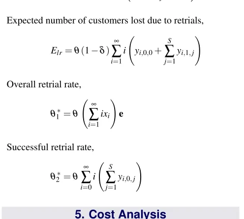
Expected number of customers lost due to retrials,

Elr=θ(1−δ) ∞

∑

i=1

i yi,0,0+

S

∑

j=1

yi,1,j

!

Overall retrial rate,

θ₁∗=θ

∞

∑

i=1

ixi

! e

Successful retrial rate,

θ₂∗=θ

∞

∑

i=0

i

S

∑

j=1

yi,0,j

!

5. Cost Analysis

we define the expected total cost per unit time as

C(s,S) =(CF+ (S−s)c1)Ero+c2Einv+c3Eorbit

+c4(Elb+Elr) +c5Eds+c6Ep

where,CF=fixed cost,c1=procurement cost per unit per unit

time, c2=holding cost of inventory per unit per unit time,

c3=holding cost of customers per unit per unit time,c4=cost

due to loss of customers per unit per unit time,c5=cost due to

service per unit per unit time,c6=cost due to decay of items

per unit per unit time.

5.1 Numerical Results and Interpretations

The following tables represent the effect of variation different parameters on the overall and successful rate of retrials

Table 1.Variation inλ λ θ₁∗ θ₂∗

2.0 1.4098 0.080379

2.1 1.5070 0.086583

2.2 1.6075 0.093005

2.3 1.7111 0.099638

2.4 1.8179 0.106470

2.5 1.9276 0.113490

2.6 2.0403 0.120700

2.7 2.1557 0.128070

2.8 2.2738 0.135600

2.9 2.3945 0.143280

(4)

Table 2.Variation inµ µ θ₁∗ θ₂∗

3.0 1.4098 0.080379

3.1 1.3881 0.080238

3.2 1.3676 0.080114

3.3 1.3483 0.080005

3.4 1.3302 0.079909

3.5 1.3131 0.079826

3.6 1.2969 0.079754

3.7 1.2817 0.079692

3.8 1.2672 0.079639

3.9 1.2535 0.079595

Fix(S,s,λ,ω,β,θ,γ,δ) = (20,5,2,0.3,1.5,1.2,0.7,0.6)

Table 3.Variation inω ω θ₁∗ θ₂∗

0.3 1.4098 0.080379

0.4 1.4104 0.081409

0.5 1.4136 0.082939

0.6 1.4202 0.084894

0.7 1.4302 0.087203

0.8 1.4438 0.089797

0.9 1.4609 0.092604

1.0 1.4813 0.095555

1.2 1.5049 0.098588

Fix(S,s,λ,µ,β,θ,γ,δ) = (20,5,2,3,1.5,1.2,0.7,0.6)

Table 4.Variation inβ β θ₁∗ θ₂∗

1.1 1.4275 0.095610

1.2 1.4202 0.090481

1.3 1.4153 0.086416

1.4 1.4120 0.083116

1.5 1.4098 0.080379

1.6 1.4084 0.078063

1.7 1.4075 0.076072

1.8 1.4069 0.074335

1.9 1.4066 0.072799

Fix(S,s,λ,µ,ω,θ,γ,δ) = (20,5,2,3,0.3,1.2,0.7,0.6)

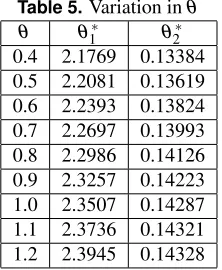
Table 5.Variation inθ θ θ₁∗ θ₂∗

0.4 2.1769 0.13384

0.5 2.2081 0.13619

0.6 2.2393 0.13824

0.7 2.2697 0.13993

0.8 2.2986 0.14126

0.9 2.3257 0.14223

1.0 2.3507 0.14287

1.1 2.3736 0.14321

1.2 2.3945 0.14328

Fix(S,s,λ,µ,ω,β,γ,δ) = (20,5,2.9,3,0.3,1.5,0.7,0.6)

Table 6.Variation inγ γ θ₁∗ θ₂∗

0.1 0.17556 0.007849

0.2 0.35950 0.016904

0.3 0.55190 0.027191

0.4 0.75293 0.038710

0.5 0.96276 0.051439

0.6 1.18160 0.065344

0.7 1.40980 0.080379

0.8 1.64760 0.096491

0.9 1.89510 0.113630

Fix(S,s,λ,µ,ω,β,θ,δ) = (20,5,2,3,0.3,1.5,1.2,0.6)

Table 7.Variation inδ δ θ₁∗ θ₂∗

0.1 0.9167 0.043151

0.2 0.9833 0.047769

0.3 1.0613 0.053363

0.4 1.1542 0.060268

0.5 1.2675 0.068996

0.6 1.4098 0.080379

0.7 1.5967 0.095891

0.8 1.8592 0.118510

0.9 2.2750 0.155740

Fix(S,s,λ,µ,ω,β,θ,γ) = (20,5,2,3,0.3,1.5,1.2,0.7)

The number of customers in the orbit increases when

the arrival rateλ increases. From table 1, it is clear that

the overall and successful rate of retrials increase with the

increase inλ. From table3, ifωincreases then the inventory

level reduces due to decay, the overall and successful rates of retrials increase because the number of customers in the

orbit gets increased. The increase in either the service rateµ

or the replenishment rateβ, the number of orbiting customers

get decreased so that the overall and successful rate of retrials

decrease (see tables2,4). When the probabilitiesγ andδ

increase, the number of customers in the orbit also increases so that the overall and successful rate of retrials from the orbit

increase. (see tables6and7). It is obvious that asθincreases,

the overall and successful rate of retrials also increase. (see

table5).

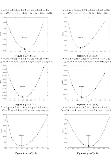
5.2 Graphical Illustrations and Interpretation

The optimum value of the expected total cost per unit time by varying the parameter one at a time and keeping others fixed. Here, we fixed maximum inventory level as 20 unit and reorder level as 5 unit. By fixing all the parameter except the arrival

rateλ. It is clear from fig.1that the cost function attains its

minimum value 131.8 atλ=2.5. As perishable rate increases

and keeping other parameters fixed, one can observe that the

cost function attains the minimum value 145.05 atω=0.4

(see fig.3). One can also observe the minimum value of the

objective function by changing other parametersµ,β,θ,γand

(5)

µ=3;ω=0.3;β=1.5;θ=1.2;γ=0.7;δ =0.6; CF=20;c1=1;c2=12;c3=c4=c5=1;c6=0.01;

Figure 1.λ vsC(s,S)

λ=2;ω=0.3;β=1.5;θ=1.2;γ=0.7;δ =0.6; CF=20;c1=c2=1;c3=6.3;c4=1;c5=0.1;c6=1;

Figure 2.µvsC(s,S)

λ=2;µ=3;β =1.5;θ=1.2;γ=0.7;δ=0.6; CF=20;c1=1.1;c2=13;c3=c4=c5=c6=1;

Figure 3.ω vsC(s,S)

λ=2;µ=3; ;ω=0.3;θ=1.2;γ=0.7;δ =0.6; CF=20;c1=c2=1;c3=46;c4=1;c5=3;c6=1;

Figure 4.β vsC(s,S)

λ=2;µ=3;ω=0.3;β=1.5;γ=0.7;δ=0.6; CF=20;c1=c2=c3=c4=1;c5=0.01;c6=1;

Figure 5.θvsC(s,S)

λ =2;µ=3;ω=0.3;β=1.5;θ=1.2;δ =0.6; CF=20;c1=4;c2=c6=1;c3=2.3;c4=1;c5=0.01;

(6)

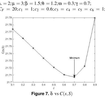
λ=2;µ=3;β =1.5;θ=1.2;ω=0.3;γ=0.7;

CF = 20;c1 = 1;c2 = 0.6;c3 = c4 = c5 = c6 = 1;

Figure 7.δ vsC(s,S)

6. Concluding remarks

We studied a continues review perishable inventory sys-tem with exponentially distributed service time and lead time. We assumed that the inter arrival time of customers follows exponential distribution. The successful rates of retrial out of all retrials were tabulated. The minimum values of the expected total cost for the variations of different parameters were illustrated graphically. One can extend this model by considering the changes in the arrival process or service time distribution.

References

[1] _{S Kalpakam and S Shanthi. A perishable inventory}

sys-tem with modified (s- 1, s) policy and arbitrary processing

times. Computers & Operations Research, 28(5):453–

471, 2001.

[2] _{R Jayaraman, C Alexander, and G Arivarignan.}

Perish-able inventory system with postponed demands and

im-patient customer.International Journal of Mathematics,

Game Theory, and Algebra, 21(2/3):161, 2012.

[3] _{K Jeganathan, N Anbazhagan, and B Vigneshwaran.}

Per-ishable inventory system with server interruptions,

mul-tiple server vacations, and n policy. International

Jour-nal of Operations Research and Information Systems (IJORIS), 6(2):32–52, 2015.

[4] _{S Kalpakam and G Arivarignan. A continuous review}

perishable inventory model. Statistics, 19(3):389–398,

1988.

[5] _{R Jayaraman, B Sivakumar, and G Arivarignan. A}

per-ishable inventory system with postponed demands and

multiple server vacations.Modelling and Simulation in

Engineering, 2012:8, 2012.

[6] _{B Sivakumar. A perishable inventory system with retrial}

demands and a finite population. Journal of

Computa-tional and Applied Mathematics, 224(1):29–38, 2009.

[7] _{O Berman and KP Sapna. Optimal service rates of a}

service facility with perishable inventory items. Naval

Research Logistics (NRL), 49(5):464–482, 2002.

[8] _{C Periyasamy. A finite population perishable inventory}

system with customers search from the orbit.

Interna-tional Journal of ComputaInterna-tional and Applied

Mathemat-ics, 12(1):2017.

[9] _{Agasi Zarbali ogly Melikov, Leonid A Ponomarenko,}

and Mamed Oktay ogly Shahmaliyev. Models of perish-able queueing-inventory system with repeated customers.

Journal of Automation and Information Sciences, 48(6), 2016.

[10] _{Jesus R Artalejo, A Krishnamoorthy, and Maria Jesus}

Lopez-Herrero. Numerical analysis of (s, s) inventory

systems with repeated attempts. Annals of Operations

Research, 141(1):67–83, 2006.

[11] _{Jesus R Artalejo. A classified bibliography of research}

on retrial queues: progress in 1990–1999.Top, 7(2):187–

211, 1999.

[12] _{Jesus R Artalejo. Accessible bibliography on retrial}

queues: Progress in 2000–2009.Mathematical and

com-puter modelling, 51(9-10):1071–1081, 2010.

[13] _{Gennadij Falin. A survey of retrial queues.} _Queueing

systems, 7(2):127–167, 1990.

[14] _{A Krishnamoorthy and KP Jose. Comparison of}

inven-tory systems with service, positive lead-time, loss, and

retrial of customers. International Journal of Stochastic

Analysis, 2007, 2007.

[15] _{Marcel F Neuts and BM Rao. Numerical investigation of}

a multiserver retrial model.Queueing systems, 7(2):169–

189, 1990.

[16] _{Gennadi Falin and James GC Templeton.} _{Retrial queues}_,

volume 75. CRC Press, 1997.

[17] _{Richard L Tweedie. Sufficient conditions for regularity,}

recurrence and ergodicity of markov processes. In

Math-ematical Proceedings of the Cambridge Philosophical Society, volume 78, pages 125–136. Cambridge Univ Press, 1975.

? ? ? ? ? ? ? ? ? ISSN(P):2319−3786 Malaya Journal of Matematik

A queueing-inventory system with perishable items and retrial of customers