Scene Classification using Localized Histogram of Oriented Gradients Method

(1)

(IJC)

ISSN 2307-4523 (Print & Online)

http://ijcjournal.org/

Scene Classification Using Localized Histogram of

Oriented Gradients Method

Md. Faisal Bin Abdul Aziz

a

*, Machbah Uddin

b

, Mohammad Khairul Islam

c

a_{Comilla University, Kotbari, Comilla 3506, Bangladesh}

b_{University of Chittagong, Chittagong, Chittagong 4331, Bangladesh}

c_{University of Chittagong, Chittagong, Chittagong 4331, Bangladesh}

a_{Email: [email protected]}

b_{Email: [email protected]}

c_{Email: [email protected]}

Abstract

Scene classification is an important and elementary problem in image understanding. It deals with large number

of scenes in order to discover the common structure shared by all the scenes in a class. It is used in medical

science (X-Ray, ECG and Endoscopy etc), criminal detection, gender classification, skin classification, facial

image classification, generating weather information from satellite image; identify vegetation types,

anthropogenic structures, mineral resources, or transient changes in any of these properties. In this paper, at first

we propose a feature extraction method named LHOG or Localized HOG. We consider that an image contains

some important region which helps to find similarity with same class of images. We generate local information

from an image via our proposed LHOG method. Then by combing all the local information we generate the

global descriptor using Bag of Feature (BoF) method which is finally used to represent and classify an image

accurately and efficiently. In classification purpose, we use Support Vector Machine (SVM) that analyze data

and recognize patterns. The basic SVM takes a set of input data and predicts, for each given input, which of two

possible classes forms the output. In our paper, we use six different classes of images.

Keywords: LHOG; Localized HOG; BoF; Scene Classification; Corner Detection.

--- * Corresponding author.

(2)

1.Introduction

A scene refers to the place where an action or event occurs. It is different from object or texture which depends

on the distance between the observer and the target point. If the distance is low that means high coverage of

point, it is called an object but when the distance increases, the fixed point goes to large scale and it is known as

scene. Images of computer, monitor, human, bus, truck etc are objects. On the other hand, an image of football

field, cricket field, bus terminal, horizon, river, mountain, forest, full image of a train etc are known as scenes.

Scene classification is a problem and great interest on researcher. Scene images have large varieties. A scene

may vary on scale, rotation, illumination another variation on two dimensional (2D) and three dimensional (3D).

Existing features that are use for scene classification are base on only color, shape, texture and other visual

parts of the image. Most of them are single descriptor. Those descriptors are single feature based and cannot

show high accuracy and effectiveness. So, we have propose a new approach which at first chooses some

interesting parts of an image that helps to find similarity between same class of images and also help to differ

from other classes of image. We propose a method for selecting interest in an image which is used to decide

locally important patches. After selecting the points we analyze the surrounding area of that point and apply a

method to generate Localized feature which we name as LHOG feature. Then we convert all local features,

LHOG, to global feature and thus get a final descriptor of an image. Then we apply Support Vector Machine

(SVM) to train itself and then classify the descriptor from a test image. We have found a global descriptor that

means global feature from local features (LHOG feature) using Bag-of-features (BoF) technique [7]. As the

same way, finally we get different global descriptors. Our method makes huge variety for different classes of

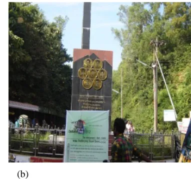
data set as example of our sample data set shown in Figure 1.

(a) (b)

Figure 1: Sample image (a) CU road (b) Zero point

HOG [6] is based on evaluating well-normalized local histograms of image gradient orientations in a dense grid.

The basic idea is that local object appearance and shape can often be characterized rather well by the

distribution of local intensity gradients or edge directions, even without precise knowledge of the corresponding

gradient or edge positions. In [16] [17] a method was developed for distinctive, scale and rotation invariant

(3)

features of images that can be use to perform matching between different views of an object or scene. A

generative model from the statistical text literature here applied to a bag of visual words representation for each

image, and subsequently, training a multi way classifier on the topic distribution vector for each image [18].

Shape and appearance based image classification that shows accuracy rate [15] but our proposed approach show

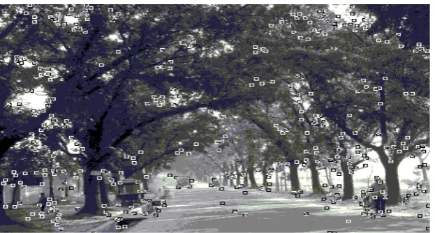
better result than others. Applying our method we see that for Figure 1(a). there are 305 corners and there

corresponding LHOG features by comparing all of these LHOG feature global descriptor is generated that is

47,51,29,11,21,48,5,16,51,26 and for Figure 1(b). there are 291 corners gives a final global descriptor

15,27,44,4,17,69,24,26,40,26. It shows that a global descriptor using LHOG value there is huge difference

between Figure 1 (a) and (b). For this reason we have achieved a good accuracy and it gives faster result.

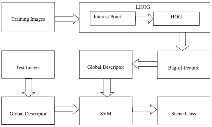
2.Proposed Method

Our method consists of the stages key point detection, feature extraction, global mapping and classification. In

the key point detection stage, we are concerned about localizing the highly informative patches. These points are

detected following the sequence of edge detection, curve extraction and finding cornerness. Around each

interest point a rectangular patch is analyzed to get statistical attributes which aims to produce local features at

that area. These local features are mapped to a multi-dimensional space in order to generate a global signature of

a scene. In our approach we use state of art Canny edge detection technology which is followed by curvature

scale space corner detector [1] method for measuring cornerness. Corner distribution in every local patch is

analyzed by constructing a normalized histogram. This histogram gives the logical feature in our method. All

logical features throughout of a given scene image are fed into the bag-of-features aiming to generate the global

signature of this scene. We use support vector machine (SVM) as our classification system. Localized HOG or

LHOG is a feature descriptor use in computer vision and image processing for the purpose of object detection

and scene classification. The technique counts occurrences of gradient orientation in localized portions of an

image. It is computed on a dense grid of uniformly spaced cells and uses overlapping local contrast

normalization for improved accuracy. Figure 2 depicts our proposed approach. The following sections illustrate

the sequence of stages in our proposed method.

3.Interest point

Interest points or corners are very vital part of an image processing technique. Interest points are located using

the following step by step procedures.

3.1.Edge Detection

Edge consists of a meaningful feature and contains significant information of an image. The edge detection

process serves to simplify the analysis of images by drastically reducing the amount of data to be processed,

while at the same time preserving useful structural information about object boundaries. In our method, we used

Canny detection method. Steps of Canny edge detection method [9][10] as follows:

a) Image Smoothing with Guassian image smoothing based on this equation

(4)

Figure 2: Overall design of scene classification.

g

( )

m,

n

=

G

σ

( ) ( )

m,

n

∗

f

m,

n

(1)

where _

    − 2 2 2σ exp 2 1 2 2

σ m +n

πσ =

G and (

m

,

n

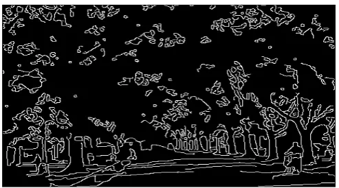
) is the pixel coordinate.

After applying Gaussian smoothing we find the image shown in Figure 3.

Figure 3: Smoothing image after Gaussiaan filter.

b) Compute the gradient magnitude from x, y partial derivatives

[

]

T

y x T

S

y

S

x

S

_

=











∂

=

∇

(2)

This is the derivatives of pixel (x,y)

Test Images

Training Images Interest Point

(5)

Gradient magnitude and orientation are as follows 2 2 y x

S

=

+

∇

(3)

x y

S

1

tan

−

=

θ

c) Apply non-maxima suppression to gradient magnitude for thinning image to eliminate non-important

edge point. Suppress the pixels in gradient which are not local maxima.

( )

_{( )}

(

₍

)

₎











′′

∇

>

∇

′

∇

>

∇

=

otherwise

0 ,

,

&

,

if

,

_S

_x

_y

_S

_x

_y

y

x

S

y

x

S

y

x

S

y

x

G

(4 )

Where

(

x

′

,

y

′

)

and

(

x

′′

,

y

′′

)

are

the

neighbors

of

( )

x,y

in

∇

S

along

the

direction

normal

to

an

edge

After applying these steps on our sample image then we get an edge map shown in Figure 4.

Figure 4: Edge-map

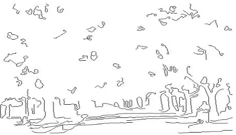
3.2.Curve Extraction and Corner Detection

Curvature is the amount by which a geometric object deviates from being flat, or straight in the case of a line,

but this is defined in different ways depending on the context. Let the equation for curvature K is

( )

( ) ( )

( )

[

₂ ₂

]

3/2

σ

u,

Y

+

σ

u,

X

σ

u,

Y

σ

u,

X

σ

u,

Y

σ

u,

X

=

σ

u,

K



₋

(5)

where

X



( ) ( )

u,

σ

=

x

u

⊗

g



( )

u,

σ

,

X



( ) ( )

u,

σ

=

x

u

⊗

g



( )

u,

σ

,

Y



( ) ( )

u,

σ

=

y

u

⊗

g



( )

u,

σ

,

( ) ( )

u,

σ

=

y

u

g

( )

u,

σ

Y



⊗



, and

⊗

is a convolution operator, while

g

( )

u,

σ

denotes a Gaussian of Width

σ

and

g



( )

u,

σ

and

g



( )

u,

σ

are the first and second derivatives of

g

( )

u,

σ

respectively [1]. After curve

(6)

extraction we get a output shown in Figure 5.

Figure 5: Extracted curve.

Now list of corner candidates are

A

j

=

{

P

_1,j

P

_2,.j

....

P

_Nj

}

where

P

_ij

=

{

x

_ij

,

y

_ij

}

are pixels on the contour. And N is the number of pixels on the contour.

Now it is either close or open

A

j is closed if

| |

P

₁j

P

_Nj

<

T

and it is open if

| |

P

₁j

P

_Nj

>

T

usually T is 2 or 3.

The contour convolved with the Gaussian smoothing kernel g is denoted by

A

_smoothj

=

A

j

⊗

g

where g is a

digital Gaussian function with width controlled by

σ

now the curvature value of each pixel value is computed

by

( ) ( )

[

₂ ₂

]

3/2 2 2 j i j i j i j i j i j i j i

Δy

+

Δx

Δy

x

Δ

y

Δ

Δx

=

K

−

for i=1,2,3,... . .. . , N (6)

where

Δx

_ij

=

(

x

_i₊j₁

−

x

_ij₋₁

)

/

2

,

Δy

_ij

=

(

y

_i₊j₁

−

y

_ij₋₁

)

/

2

and

(

)

/

2

2 j 1 i j 1 + i j

i

=

Δx

x

Δ

−

− , 2

(

ij1

)

/

2

j 1 + i j

i

=

Δy

y

Δ

−

− and all the local maximum and curvature function

are included in the initial list of corner candidates. But there may be some rounded corners that’s needed to

remove. We can remove it by adaptive threshold methods [2].

( )

_∑

|

( )

|

−

×

1 L u = i 2

L

+

u

i

K

+

L

+

L

R

=

K

R

=

u

T

2 1

1

(7)

where u is the position of the corner candidate and

L

₁

+

L

₂ is the position of the ROS centre at u and R is a coefficient. After applying curvature extraction, round corner and false corner removing [1], then we get our

desire interest points as shown Figure 6.

4.Feature Extraction

In a scene image, we can observe that the most of the area belonging to this scene is flat. Generally a flat area

does not contain enough clues to represent the image in a discriminative way. Rather the textured area is very

(7)

good at representing the scene contents. Considering this in our mind, we try to select a patch around the corner

points which are treated as interest point in the previous section. The selected patch area is shown in Figure 7.

Figure 6: Detected corner. The small rectangle denotes the small patch around the corner.

Figure7: Patch area.

4.1 Localized Feature

In this method we consider that every part as an interesting point that is a local representation of that point. In

each scene, we separate an interesting point by corners and there corresponding HOG [3] [6] value around the

corners. After corner detection generating HOG values that makes a Localized HOG or LHOG feature as

follows:

LHOG feature = Interest point + Corresponding HOG of interest point (8)

Our sample image there is 305 important corners are detected. For example a corner point (255, 31) is selected

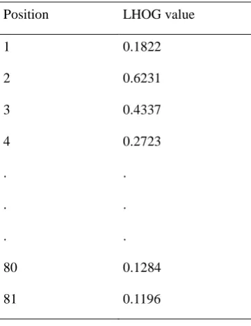
and its patch area is 25 X 50 pixels. LHOG values of Figure 7 are shown in table 1.

4.2 Global Mapping

Global mapping represents the over structure and distribution of local features. To perform this we use

bag-of-features. BoF approaches are characterized by the use of an orderless collection of image bag-of-features. Lacking any

structure or spatial information, it is perhaps surprising that this choice of image representation would be

(8)

powerful enough to match or exceed state-of-the-art performance in many of the applications to which it has been

applied [7]. BoF generates global feature from all of the local features. In our method all the LHOG value are

combined and after applying clustering method we generates a global descriptor. Bag-of-Feature takes the

following steps shown as Figure 8.

Table 1: LHOG values for an interested point

Position LHOG value

1 0.1822

2 0.6231

3 0.4337

4 0.2723

. .

80 0.1284

81 0.1196

The rest of corners generate 81 X 1 matrix of LHOG descriptor. All of the LHOG values are considered as a

local descriptor.

Figure 8: Stepwise Bag-of-Feature.

First LHOG value is compared with all 10 cluster and find the minimum distance it goes to cluster 2 finally we

got a global descriptor based on 305 LHOG value. Global descriptor from LHOG using K means clustering [5].

Finally we applied this method for all of images of same class and different 6 classes. Image representation by

codeword [4] using LHOG frequencies shown in Figure 9.

(9)

Figure 9: Codewords from sample image.

5.Classification

Classification is a model that receives data as input and predicts for a given input in which class it is. In case of

supervised learning we have to provide a training data set with its group number. Then provides an input to test

in which class its similar to that input. In our case we have used Support Vector Machine [8] supervised learning

as a classifier. At first trains the SVM machine with all the images that are for training purpose actually it takes

a descriptor set and image group number. During the time of classify it takes on a test image descriptor that is

matches with trained image set. It returns a group number in which group it is more similar. It returns nothing if

it is not closely match with none of group.

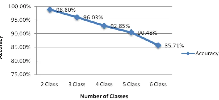
6.Experimental Result

In our research there are 6 classes of data set and we applied stratified k-fold cross-validation [13]. Results are

shown in table 2 and accuracy graph in Figure 10.

Figure 10: Accuracy vs. Number of class

(10)

Table 2: Accuracy results for 2 fold cross validation.

Number

of Class

Classes Name Number of

Image per

Class

Total

Number of

Image

Number of

Image Correctly

Identified

Number of

Image Wrong

Classified

Accuracy

2 Class CU Road, IT Building 42 84 83 1 98.80%

3 Class CU Road, IT Building,

Freedom Sculpture

42 126 121 5 96.03%

Freedom Sculpture,

Shah Jalal Hall

42 168 156 12 92.85%

Freedom Sculpture,

Shah Jalal Hall, Saheed

Minar

42 210 190 20 90.48%

Freedom Sculpture,

Shah Jalal Hall, Saheed

Minar, Zero Point

42 252 216 36 85.71%

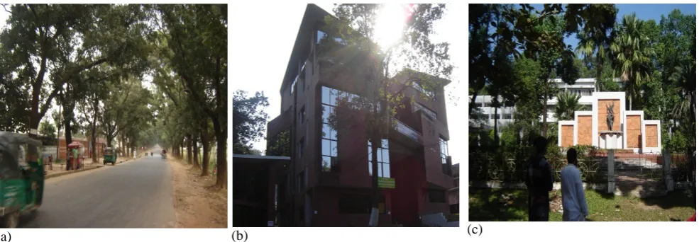
Our dataset is self data set shown in Figure 11.

(a) (b) (c)

(11)

(d) (e) _(f)

Figure 11: Sample images of our data Set where (a) CU Road, (b) IT Building, (c) Freedom Sculpture, (d)

Saheed Minar, (e) Shah Jalal Hall, (f) Zero Point.

6.1.Recall and Precision Graph

In pattern recognition precision [12] is the fraction of retrieved instances that are relevant, while recall is the

fraction of relevant instances that are retrieved. Both precision and recall are therefore based on an

understanding and measure of relevance. When referring to the performance of a classification model, we are

interested in the model’s ability to correctly predict or separate the classes. When looking at the errors made by

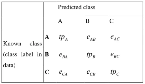
a classification model, the confusion matrix gives the full picture. Considering three classes problem with A, B,

and C class. A predictive model may result in the following confusion matrix when tested on independent data.

The confusion matrix shows how the predictions are made by the model in table 3.

Table 3: Confusion matrix with notation

Predicted class

A B C

Known class

(class label in

data)

A

tp

_A

e

_AB

e

AC

B

e

_BA

tp

_B

e

BC

C

e

_CA

e

_CB

tp

_C

i) Precision:

Precision is a measure of the accuracy provided that a specific class has been predicted.

It is defined by:

Precision

=

tp

/

(

tp

+

fp

)

(9)

(12)

where

tp

and

fp

are the numbers of true positive and false positive predictions for the considered class. In the

confusion matrix above, the precision for the class A would be calculated,

Precission

A

=

tp

A

/

(

tp

A

+

e

BA

+

e

CA

)

=

25 /

(

25 +

3 +

1 )

≈

0.86

(10)

ii) Recall:

Recall is true positive rate. It is defined by the formula:

Recall

=

Sensitivit

y

=

tp

/

(

tp

+

fn

)

(11)

where

tp

and

fn

are the numbers of true positive and false negative predictions for the considered class.

fn

+

tp

is the total number of test examples of the considered class. For class A in the matrix above, the recall

would be:

(

)

(

25

5

2 )

≈

0.78 /

25 /

+

=

e

+

e

+

tp

=

y

Sensitivit

=

Recall

_A _A _A _A _AB _AC

(12)

Our experimental result of recall and precision in various classes are shown in Figure 12.

6.2.Receiver Operating Characteristics (ROC)

ROC [11] [12] curve is a useful technique for organizing classifiers and representing their performance. It is

created by plotting the fraction of true positive rate (TPR) vs. false positive rate (FPR). Let us define an

experiment from P positive instances and N negative instances. The four outcomes can be formulated in a 2×2

confusion matrix in table 4.

Table 4: Confusion matrix for ROC curve

The calculation of TPR and FPR are as follows:

TPR

=

TP

/

P

=

TP

/

(

TP

+

FN

)

(13)

FPR

=

(

FP

/

N

)

=

FP

/

(

FP

+

TN

)

(14) Prediction outcome

Actual value

P' N' Total

P True Positives False Negatives P

N False Positives True Negatives N

Total

P' N'

(13)

(a) (b)

(c) (d)

(e)

Figure 12: Recall precision graph for (a) 2 class (b) 3 class (c) 4 class (d) 5 class (e) 6 class.

Our experimental results of 2 fold ROC curve for different number of scene classes are as shown in Figure 13.

7.Conclusion and Future Work

In this paper we propose a novel scene classification method. our research we have achieved a good

performance that on previous graph and its accuracy rate is high that is above 85 percent. Our database contains

images in variety of format on same class.

(14)

(a) (b)

(c) (d)

(e)

Figure 13: ROC curve for (a) 2 class (b) 3 class (c) 4 class (d) 5 class (e) 6 class.

(15)

Total time of classifying scene that includes input data to classified output is 31.8837s and it was for 84 images

hence per image computation time is

31.8837

/

84 =

0.3796

s where image resolution was 461× 365 pixels. This time is slower than other existing system of scene classification also our accuracy is higher than other

existing systems of scene classification.

In future we will concentrate on increasing accuracy and reducing processing time. We will try to obtain

processing time 0.05s per image so that our proposed method can work in security system such as criminal

detection from video.

References

[1] X.C. He. and N.H.C. Yung. “Curvature scale space corner detector with adaptive threshold and dynamic region of support.” International conference on pattern recognition, Vol. 2, pp 791-794, 2004.

[2] X.C. He. and N.H.C. Yung. “Corner detector based on global and local curvature properties.” Optical engineering,vol. 47, no. 5, pp. 057008(1-12), 2008.

[3] O. Ludwig, D. Delgado, V. Goncalves and U. Nunes. “Trainable classifier-fusion schemes: an application to pedestrian detection.”Conference on intelligent transportation systems, vol. 1, pp 432-437, 2009.

[4]

Cordelia Schmid. Class Lecture, Topic: “Bag-of-features for category recognition.” Paris, Sep. 4, 2013.

[5

] K. Teknomo. “Numeric example of k-means clustering.” Internet:

http://www.people.revoledu.com/kardi/tutorial/kMean/NumericalExample.htm, [Nov. 29, 2013].

[6]

N. Dalal and B. Triggs. “Histograms of oriented gradients for human detection.” IEEE computer sciety conf.erence on computer vision and pattern recognition, vol. 1, pp. 886-893, 2005.

[7] O. Stephen and A.D. Bruce. “Introduction to the bag of features paradigm for image classification and retrieval.” Computing research repository, vol. arXiv:1101.3354v1, 2011.

[8]

Y. Lee, Y. Lin,and G. Wahba. "Multicategory support vector machines: theory and application to the classification of microarray data and satellite radiance data.” Journal of american statistical association, vol. 99 (4655), pp. 67-81, 2004.

[9]

B. Green “Canny Edge Detection Tutorial.” Internet: http://www.scribd.com/doc/40036113/Canny-Edge-Detection-Tutorial, 2002 [Nov. 01, 2015].

[10] R.

Wang

. “Canny edge detection.” Intenet: http://fourier.eng.hmc.edu/e161/lectures/canny/node1.html, Sep. 25, 2002 [Nov. 01, 2015].

[11] J. Fogarty, R.S. Baker and S.E. Hudson. “Case studies in the use of ROC curve analysis for sensor-based estimates in human computer interaction” Proceedings of graphics interface, pp. 129-136, 2005.

[12] D. M. W. Powers. “Evaluation: From precision, recall and f-measure to ROC, informedness, markedness & correlation.” Journal of machine learning technologies, vol. 2(1), pp-37-63, 2011.

[13] J. Schneider. “Cross Validation. Internet: http://www.cs.cmu.edu/~schneide/tut5/node42.html, Feb. 7, 1997 [Nov. 02, 2015].

(16)

[14] R. Kohavi."A study of cross-validation and bootstrap for accuracy estimation and model selection."

Proceedings of the fourteenth international joint conference on artificial intelligence, pp 1137–1143, 1995.

[15] A. Bosch, A. Zisserman and X. Muñoz. “Image classification using random forests and ferns”.

Proceedings of Asian conference on computer vision, Tokyo, Japan, 2007.

[16] V. Andersen; L. Pellarin; R. Anderson, “Scale invariant feature transform (SIFT): performance and application”, The IT University of Copenhagen, pp, 1-14, 2006.

[17] D. G. Lowe. “Distinctive image features from scale-invariant key points”, International journal of computer vision, vol. 60, pp. 91-110, 2004.

[18] N. I. Cinbis; S. Sclaroff, “Object, scene and actions: Combining multiple features for human action recognition”, Proceeding of European conference on computer vision , 2010, pp 494-507.

[19] A. Bosch; A. Zisserman; X. Muñoz, “Scene classification using a hybrid generative/discriminative approach”, IEEE Transaction on pattern analysis and machine intelligence, vol. 30 no. 4, pp. 712-727, 2008.