An Application of SMC to continuous validation of
heterogeneous systems
Alexandre Arnold
1, Massimo Baleani
2, Alberto Ferrari
2, Marco Marazza
2, Valerio Senni
2, Axel
Legay
3, Jean Quilbeuf
3, Christoph Etzien
41[email protected], AIRBUS, Toulouse, France 2[email protected], ALES - UTRC, Roma, Italy 3[email protected], Inria, Rennes, France
4name.surname@offis.de, OFFIS, Oldenburg, Germany
Abstract
This paper considers the rigorous design of Systems of Systems (SoS), i.e. systems composed of a set of heterogeneous components whose number evolves with time. Such components cooperate to accomplish functions that they could not achieve in isolation. Examples of SoS include smart cities or airport management system. The dynamical evolution of SoS behavior and architecture makes it impossible to design an appropriate solution beforehand. Consequently, existing approaches build on an iterative process that takes SoS evolution into account. A key challenge in this process is the ability to reason about and analyze a given view of the SoS (on a fixed number of SoS constituents) with respect to a set of goals, and use the results to eventually predict the evolution of the SoS. To address this challenge, we rely on a scalable formal verification technique known as Statistical Model Checking (SMC). SMC quantifies how close the current view is from achieving a given mission. We integrate SMC with existing industrial practice, by addressing both methodological and technological issues. Our contribution is: (1) a methodology for validation of SoS formal requirements; (2) a formal specification language able to express complex SoS requirements; (3) the adoption of current industry standards for simulation and heterogeneous systems integration ; (4) a robust SMC tool-chain integrated with system design tools used in practice. We illustrate the application of our SMC tool-chain and the obtained results on a case study.
Receivedon 22 November 2017;acceptedon 18 July 2017;publishedon 21 December 2017 Keywords: Systems of systems, statistical model checking, FMI, tool-chain, simulation.
Copyright © 2017 Alexandre Arnold et al., licensed to EAI. This is an open access article distributed under the terms of the Creative Commons Attribution licence (http://creativecommons.org/licenses/by/3.0/), which permits unlimited use, distribution and reproduction in any medium so long as the original work is properly cited.
doi:10.4108/eai.21-12-2017.153500
1. Introduction
Context and challenges A System of Systems (SoS)
is a large-scale, geographically distributed set of
HResearch supported by the European Community’s Seventh Framework Programme [FP7] under grant agreement no 287716 (DANSE).
HHThis paper is an extension of the paper “An Application of SMC to continuous validation of heterogeneous systems.” published in the proceedings of the SIMUTOOLS 2016 conference.
independently managed, heterogeneous Constituent Systems (CS). The heterogeneity of CSs arise from their variations in nature, time scale, and model of computation. Constituent systems are collaborating as a whole to accomplish functions and goals that could not be achieved otherwise by any of them, if considered alone [1]. Those goals can either be global to the system or local to some of its constituents. Constituent Systems are loosely coupled and pursue their own objectives, while collaborating for achieving SoS-level objectives.
An SoS adapts itself to its environment through (1) an evolution of the functions provided by its Constituent Systems and (2) an evolution of its architecture. A typical example of an SoS is the Air Traffic Management System of an airport, which coordinates incoming and outgoing aircrafts as well as ground-based vehicles and controllers. Such an SoS may evolve in order to accommodate a larger number of passengers, difficult climatic conditions or a modification in the laws regarding security.
Misbehaviours of the functions provided by an SoS can be dangerous and costly. Therefore, it is important to identify a set of analyses and tools to verify that the SoS implementation meets functional and non functional requirements, and correctly adapts to changes of the environment during any phase of the design and operation life-cycle. The manager of a SoS should be able to run these analyses in order to take decisions regarding the evolution of the SoS.
The main characteristics of an SoS have been long debated since [1]. One of the key characteristics of an SoS is dynamical evolution, that is, the fact that Constituent Systems may evolve, leave, fail, or be replaced. In fact, dynamical evolution of SoS makes it impossible to design an appropriate solution beforehand. Consequently, the design flow of a SoS is reiterated multiple times during the operation of the SoS, in order to adapt to its evolutions.
As a summary, SoS rigorous design methodologies introduce two major challenges. The first one is to check whether a given view of the system (i.e. a fixed number of components) is able to achieve a mission. The second challenge is to exploit the solution to the first challenge in an engineering methodology that permits dynamical evolution of the system in case new missions are proposed, in case the environment has changed, or in case the current view cannot achieve the mission. This design approach has been followed by the DANSE project which developed a new SoS design and operation methodology [2].
Contributions This paper focuses on the first
chal-lenge described above, that is to reason on a given view of the system. A corner stone to solve the challenge is to develop a usable language for expressing formal requirements independent from the number and iden-tity of CSs and thus from the architectural choices.
In this paper, we propose Goals and Contracts Requirement Language (GCSL), which is an expressive pattern-based language designed to specify require-ments on an SoS and its CSs. The language uses an extension of OCL to express constraints independently of the view such as: “the total fire area (over a set of districts) is smaller than 1 percent of the total area of the districts”. By combining those constraints
with temporal patterns, we express timing require-ments on the behaviors of the view. For instance, the GCSL formula “always[SoS.itsDistricts.fireArea→sum()< 0.01∗SoS.itsDistricts.area→sum()]” checks that the above constraint is verified at any point of the simulation. A first version of GCSL was introduced in [3]. In this paper we propose additional patterns for expressing properties about the amount of time during which a given predicate remains satisfied. We show that GCSL is powerful enough to capture most of SoS goals and emergent behaviors proposed by our industry partners. The reader shall observe that the language can method-ologically be extended to capture more requirements on demand.
The second main difficulty is to detect emergent behaviors and verify the absence of undesired ones. This requires a suitable verification technique. A first solution would be to use formal techniques such as model checking. Unfortunately, both the complexity and the heterogeneous nature of the constituent systems prevent this solution. To solve this problem, we rely on Statistical Model Checking (SMC) [4]. SMC works by monitoring executions of the system, and rely on statistics to assess the overall correctness. Contrarily to classical Validation techniques, SMC quantifies how close the view is from achieving a given mission. This information shall later be exploited in the reconfiguration process.
The objective of this paper is not to improve existing statistical algorithms, but to integrate the SMC verifier PLASMA [5] into a full tool chain for verifying heterogeneous systems. PLASMA proposes several statistical algorithms such as Monte Carlo or hypothesis testing. In order to implement an SMC algorithm for SoS, one has to propose a simulation approach for heterogeneous components as well as a monitoring approach for GCSL requirements. While a GCSL monitor is easily obtained by translating GCSL to Bounded Temporal Logic (BLTL) as in [6], simulating SoS requires that one defines a formal representation for SoS constituents. In this work, we exploit the Functional Mock-up Interface (FMI) [7] standard as a unified representation for heterogeneous systems. In recent years, the development of DESYRE [8–10], a simulation engine based on the System-C standard, provided us joint simulation for FMI/FMU. One of the main contributions of the paper is a full integrated tool-chain between IBM Rhapsody, the statistical model checker PLASMA [5] and DESYRE. This tool-chain is, to the best of our knowledge, the first one offering a full SMC-based approach for the verification of complex heterogeneous systems.
The third main difficulty of our work is to make sure that the technology will be accepted by practitioners, both in terms of usability and seamless integration with existing industrial practice and tools. Our
2 Industrial Networks and Intelligent SystemsEAI Endorsed Transactions on
first contribution provides a solution for expressing requirements. However, we need a language to specify the system itself. In this paper, we propose to support wide-spread industry standards for SoS. This is done by exploiting UPDM [11] for SoS architecture design and the FMI standard for constituent systems integration. We build on IBM Rhapsody which is a tool used to describe UPDM views, that we enrich with probability distributions. Using probability distributions allows the designer to abstract away complex behaviors as well as model inputs from the environment, failure of components, and in general phenomena for which a probabilistic description is known. Finally, once the model is fully designed, an integrated tool-chain with a single GUI enables the simulation and verification of the model.
Our approach is illustrated on a fire emergency response SoS, at the scale of a city. The constituent systems are the districts of the city, firefighting cars, firemen, fire stations and the central command center. We show how our tools are used to model the architecture and the constituents systems of the SoS. The architecture indicates how the Constituent Systems cooperate to provide an emergent behavior, namely the extinction of the fires. Using our tool-chain, we evaluate the probability of this emergent behavior.
Structure of the paper The paper is organized as
follows. In Section 2, we present the modeling of SoSs. We then explain in Section 3 how to produce a simulation trace from the models. In Section 4 we provide a summary of the Statistical Model Checking approach adopted in our tool-chain. Following this, in Section 5 we introduce the GCSL formal language for specifying formal requirements on SoS and CSs behavior. Finally, we discuss in Section 6 the SMC tool-chain and its integration with existing industrial tools for System design. This tool-chain is demonstrated on an industrial case study in Section 7, where we show its application to a Fire Emergency Response system designed in DANSE [12], modeling a complex SoS that manages fire emergencies in a large city.
2. SoS Modelling
A SoS model consists of a model of the SoS architecture and a set of models formalizing each Constituent System’s behavior. We chose the UPDM language to describe both the SoS architecture and Constituent System’s behavior, even though the latter can be described through other modelling languages, as explained in the following.
UPDM, or Unified Profile for DoDAF1 and MoDAF2 [11], is a modeling language standardized by the Object Management Group (OMG) in 2012. UPDM 2.0 defines a UML 2 and optional SysML profile to model architectures, support analysis, specification, design and verification for a broad range of complex systems, including SoS architectures and service oriented architectures. Through the profile
extension mechanism inherited from UML, UPDM allows adding, extending and customizing standard profiles by creating libraries of new components and
stereotypes to further refine domain-specific concepts. A stereotype defines how an existing UML, SysML or UPDM metaclass can be extended. It can be applied to a configurable set of model elements i.e. for replacing existing features or for enabling new ones. A stereotype can have properties, referred to astagsdefinitions [13]. When a stereotype is applied to a model element, the value of the tags can be set for that model element. The remaining of this Section describes how we extended UPDM to accomplish architectural and behavioural representations of SoSs supporting statistical model checking analysis.
2.1. Modelling Constituent Systems’ Behaviour
In order to model an SoS, we need to specify the behavior of each of the constituent systems. In order to perform SMC, the model needs to exhibit a stochastic behaviour. Typical examples when stochastic behaviours are relevant in a model include formalizing variability of external inputs and waiting time before events’ occurrence, unpredictability of components’ failure, and so on.
In our approach we leave total freedom to the CS designer to use any modelling language, provided that the modelling tool implementing that language is able to export the CS model according to the FMI 1.0 standard [7]. To introduce a stochastic behavior, the designer can use functions provided by the specific tool used for modelling.
UPDM is one of the tool that can be used to model constituent systems. In that context the designer can rely on a DANSE extension to the UPDM profile developed specifically for statistical model checking. We have defined the«Stochastic» profile with a set of ad-hoc stereotypes to support stochastic variables in SV-10b viewpoint (state-charts), the UPDM view we use to model CS behaviours. Our stochastic profile defines Uniform, Normal and CustomDistribution distributions stereotypes on the Integer and Real domains; custom distribution variables are based on user-defined probability distribution functions (further
details can be found in [3]); each of the two “Uniform” stereotypes (for Integer and Real values respectively) has two tags to specify the min and max bounds of the range interval, whereas each of the two Normal stereotypes has two tags to specify the desiredmeanand
standard deviationparameters.
Again, UPDM is not the only language we support to model Constituent Systems’ behaviour. Some languages are tailored for modeling specific physical phenomena, while some others are tailored to model control systems. The designer is free to use the language that best fits the system to describe, as long as the language can export to FMI.
2.2. Modeling the architecture
The architecture of the SoS specifies how instances of constituent systems are interconnected. An SoS does not have a fixed number of CS instances over its execution because CSs are independently managed and may decide to leave or join a given SoS on their own. Therefore, rather than defining exactly how many CS are present in the SoS, we first specify an abstract architecture that defines the kind of CSs that compose the system and how they can interconnect with other CSs. For simulation, we fix a concrete architecturethat is a possible instance of the abstract architecture. Our need for describing the architecture is satisfied by the UPDM 2.0 System Viewpoint 1 (SV-1).
The SoS Abstract Architecture. The abstract architecture is specified using the SV-1 Block Definition Diagram (BDD), a representation of the SoS hierarchy defining:
1. the System of Systems and its parameters,
2. the type of each Constituent System,
3. the interface in terms of ports and their type of each Constituent System,
4. the CS parameters, along with their types and default value, and
5. the composition relations between the SoS and its CSs.
Each type of Constituent System that can participate in the SoS should be materialized in the abstract architecture by a«System» block. This block specifies the expected parameters and state variables for a constituent system of that type. It also defines the default parameters for CSs of that type. Of course, the model of the CS given to the simulator has to conform to the description given by the«System» block in the abstract architecture.
The SoS Concrete Architecture. In order to define the concrete architecture, we rely on the SV-1 Internal Block Diagram (IBD), an integration view of the SoS defining:
1. a set of instances of CS types specified in the SoS abstract architecture,
2. the role of each CS instance in the SoS, including instance-specific parameter assignments, and
3. the connections between ports of CS instances, according to the abstract architecture.
An instance of a «System» block specified in the SoS abstract architecture (UPDM SV-1 BDD) is materialized by a «ResourceRole» block in the SoS concrete architecture (UPDM SV-1 IBD). TheValuetag of UPDM
Attributes of each instance can be defined to the default parameters set in the abstract architecture (BDD) or overridden for each instance of the concrete architecture (IBD).
Besides the«Stochastic» profile described in Section 2.1, we defined two other profiles to provide informa-tion for joint simulainforma-tion and to express requirements. With these three profiles we can specify all the infor-mation needed to simulate and verify SoSs through statistical model checking.
Providing Information for Joint Simulation. To provide information for joint simulation our «Simulation» profile defines the following stereotypes: «FMI», «Traceable»and«FMIIgnore».
In order to simulate an SoS model, the simulation engine needs to load the model of each constituent system. In our case, the model of the system is an executable file (Functional Mockup Unit or FMU). The «FMI» stereotype allows the designer to link a «System»block from the abstract architecture to a FMU, by specifying an URI for that FMU. The link «FMI» stereotype can also be applied to a particular instance («ResourceRole» block) in the concrete architecture to link that instance to a specific FMU.
SMC analysis requires the observation of the SoS model variables that appear in GCSL contracts. In particular, the SMC checker will expect a trace that contains the evolution of these variables. To allow the simulation tool to properly generate observers to track values of the needed variables, we define the «Traceable» stereotype. This stereotype can be applied to any attribute of a «ResourceRole» or a «System» element to declare that the value of this attribute should appear in the output of the simulator.
Sometimes, an SoS model contains information that is not needed for a particular analysis. Filtering out such extra information to leave only the one relevant for that analysis is enabled by our«FMIIgnore» stereotype, applicable to model elements’ ports and
4 Industrial Networks and Intelligent SystemsEAI Endorsed Transactions on
attributes. When this stereotype is applied to the both ports involved in a connection, the simulator ignores that connection. Connections between ports with «FMIIgnore»applied and ports without this stereotype are not allowed. Consistently, the corresponding CS behavioural model shall not generate any data flowing through ports with the«FMIIgnore»stereotype.
Expressing Requirements. To pursue our SMC analysis goals on SoS we have defined a number of stereotypes collected by the «GoalsAndContracts» profile. One of the stereotypes of the «GoalsAndContracts» profile associates GCSL contracts to elements of the abstract architecture, possibly including the root element. To express contracts on model elements throughout our SoS UPDM SV-1 diagrams we rely on the UPDM “Constraint” model element inherited from UML [11]. To link a contract to CS or SoS «System» elements in a UPDM BDD, or to specific CS instances, stereotyped as «ResourceRole» in a UPDM IBD, we use the “constrainedElement” association provided by the “Constraint” model element. We have further extended the features of “Constraint” by defining the «gcsl» stereotype. The«gcsl»stereotype defines tags to specify (1) the GCSL assumption in textual form, (2) the GCSL guarantee in textual form, (3) the probability threshold with which the GCSL requirement has to be satisfied, and (4) the GCSL requirement identifier as an alphanumeric string.
3. Performing Joint Simulation in
DESYRE
3.1. Integrating Heterogeneous CSs’ Behaviours
Constituent Systems are systems that evolve according to their own nature and mission, independently from the SoS. The nature of the CS implies that its behaviour be modelled using the most appropriate modelling tool for the specific application, which typically leads to a set of heterogeneous format of model representation and interfaces. Formalizing different Constituent Sys-tems’ behavior requires supporting a variety of models of computation, including continuous-time dynamics, discrete-time dynamics with variable or fixed integra-tion step intervals and event-based dynamics. Very often an SoS model is composed of CS models whose integration time-step varies of several orders of magni-tude. For instance, an SoS can compose systems which act every second with systems which act every month. For these reasons we refer to a SoS model as being a composition of heterogeneous Constituent Systems’ models. To guarantee correct integration and simula-tion of heterogeneous CSs models to support statis-tical model checking we need to translate all these differences to a common format. Our approach requires CS behavioural models to comply with the Functional Mock-up Interface (FMI) [7].
A number of approaches are possible for integrating Heterogeneous CSs’ Behaviours. Co-simulation coor-dinates distinct simulation tools to provide a global simulation of the overall system. The integration can be performed using simulators’ API, a common propri-etary interface, such as the Simulink S-function, or a standard interface, for instance FMI for co-simulation. The approach proposed in this paper is based on “joint-simulation”: a single simulator integrates the models of system components (i.e. CS models in the context of this work), each consisting of differential, algebraic and discrete equations describing components’ continuous and discrete dynamics. To maximize tool interoperabil-ity the choice for a common interface to components’ equations has fallen on the one defined by the Func-tional Mock-up Interface (FMI) standard [7].
FMI is a tool-independent standard whose develop-ment was initiated within the ITEA2 project MOD-ELISAR with the objective of easing the exchange of simulation models between different entities despite the usage of a variety of different tools. FMI stan-dard was developed as a collaborative effort involving simulation tool vendors and research institutes. FMI standard maintenance and development (FMI 2.0 has been published in July 2014) is today performed by the Modelica Associations and it is currently supported by tens of academic and industrial tools.
FMI defines the interface of an executable, called Functional Mock-up Unit (FMU) and supports both model exchange and co-simulation of dynamic models. An FMU can either be self-integrating (i.e. can include its own numerical solver), or require an external simulator to perform its numerical integration. The former is the case of “FMI for co-simulation”, the latter is called “FMI for model exchange”. FMUs used for joint-simulation have to comply to the “FMI for model exchange” interface, version 1.0. This version of the interface allows handling “hybrid ODEs” [14] i.e. ordinary differential equations in state space form with events. Systems described by hybrid ODEs combine a piecewise continuous state (discontinuities occur at event instants) with a time-discrete state that changes only in correspondence of event instants.
In co-simulation, each FMU embeds its own ODE solver and computes autonomously the evolution of its continuous-time variables. In model exchange, the MA is in charge of computing evolution of continuous-time variable.
The implementation of a Master Algorithm (MA) is not a trivial task, since the algorithm has to guarantee:
1. the correctness of the composition according to the model(s) of computation (MoC) of both the host environment and the constituent FMUs,
2. the termination of the integration step and
3. the determinism of the composition.
Challenges related to the implementation of Master Algorithms for model composition, have been exten-sively addressed in the literature. In [15] the authors define the operational and denotational semantics of the (hierarchical) composition of Synchronous Reactive (SR), Discrete Event (DE), and Continuous Time (CT) models. Termination and determinacy properties of MA for co-simulation are addressed in [16].
3.2.
DESYRE
Master Algorithm
Within the context of the DANSE project a specific FMI Master Algorithm (MA) has been developed in DESYRE to address the unique needs of Systems of Systems simulation and SMC. The focus is on simulation efficiency, needed because of the SoS model complexity and large observation (i.e. simulation) time span (up to several years) as well as the large number of runs (tens or hundreds of thousands) required by the SMC analysis. The MA builds on a set of assumptions that are typically satisfied by the CS models used within the DANSE context. The choice of a MA for model exchange rather than co-simulation provides us with full control of the overall integration algorithm. The MA assumes that none of the FMUs contains direct feed-through i.e. FMU output does not depend on the value of its inputs at the current simulation time, removing the need for a causality analysis during the fixed point computation at each step. The solver used for the continuous state of continuous-time FMUs is the simple forward Euler algorithm rather than higher order Runge-Kutta (RK) methods. While this method can be numerically unstable and its global error is linear with the integration step, it does not require the computation of state (and inputs) at intermediate steps, which makes the integration method compositional and does not require any “roll-back” mechanism due to the validity of the selected step size. In the current implementation the step sizemaxIntStepis specified by the user for the entire model but can be easily extended to support a different step size for each FMU. Besides affecting the rounding error and the stability of the
Algorithm 1DESYRE FMI MA for DANSE.
Input: simStartT ime, simEndT ime, maxIntStep;
1:simT ime=simStartT ime;
2:isCT=determineIf CT();
3:for allcs∈csListdo
4: csEvt=cs.initialize(simT ime);
5: if(csEvt,∅);then
6: evtQueue.addEvt(cs.getID(), csEvt);
7: end if
8: if(((evtQueue.getClosestEvtTime()−simT ime)> maxIntStep)and isCT)
then
9: evtQueue.addEvt(cs.getID(), maxIntStep);
10: end if
11:end for
12:while(simT ime≤simEndT imeand not(simStopEvt))do
13: simT ime=getSimT ime();
14: while(not(isSoSFixP tReached()))do
15: for allcs∈csListdo
16: cs.updateDiscrState(simT ime);
17: end for
18: end while
19: for allcs∈csListdo
20: cs.updateContState(simT ime);
21: end for
22: evtQueue.updateEvts();
23: simT ime=evtQueue.getClosestEvtTime();
24: waitNextActivationEvt();
25:end while
algorithm the step size determines also the capability of detecting state events (i.e. zero-crossing) occurring during an integration step as well as their location on the time axis. In fact, state events are checked for only at the end of each integration cycle and, if detected, are given a time stamp equal to current simulation time with an error that in the worst case equals the discretization step maxIntStep. All these limitations were proven acceptable in all the use cases exercised within the DANSE project.
Lines 1 to 11 in Algorithm 1 represent the initialization phase, while lines 12 to 25 describe the SoS system simulation loop. The algorithm determines the time synchronization instants for the different FMUs composing the SoS model. Time synchronization points represent those time instants in which (1) the different FMUs are executed, (2) the generated outputs are propagated among their interfaces (line 16) and (3) FMU continuous state is updated (line 20). Synchronization points are calculated based on time events, state events and step events notified by the different FMUs [7].
3.3. Joint-Simulation Traces
The execution of a SoS model results in a trace, that is exploited by our SMC analysis. The formal definition of trace is provided by Definition 1.
Definition 1.Given a set of variablesV and their domain D, a stateσ is a valuation of the variables, that isσ ∈ DV. A trace τ is a sequence of states and timestamps (σ0, t0),· · ·,(σk, tk), where∀i ti ∈R+∧ti < ti+1.
In our setting, a trace contains an element for each time step of the simulation. At each step, the value of all
6 Industrial Networks and Intelligent SystemsEAI Endorsed Transactions on
observed variables are recorded. The observed variables
V are the exported variable to which the «traceable» stereotype has been applied.
4. Background on Statistical Model Checking
Analyzing Systems of Systems requires a careful choice of the verification technique to use. A first solution would be to use model checking. However, this formal approach often requires an input written in a dedicated language, which conflicts with industry acceptance. Even if a complete model were made in a suitable language, analysis would not be feasible because of the very large size of SoSs and its heterogeneous nature. Therefore, we rely on Statistical Model Checking (SMC), which is a trade off between testing and model checking. SMC works by simulating the system and verifying properties on the simulations. An algorithm from the statistic area exploits those results to estimate the probability for the system to satisfy a given requirement.
The quantitative results provided by SMC is richer than a Boolean one. Indeed, if the system does not satisfy the requirement, a Boolean tool returns “not satisfied” without any evaluation of the probability of a correct behavior.
In order to apply SMC, one has to assume that the behavior of the system is governed by a stochastic semantic, that is the choice of the next state in an execution depends on a probability distribution. This hypothesis shall not be seen as a drawback. Indeed, most of SoS do make stochastic assumptions on their external environment or on their hardware. In case no distribution is known, one relies on the uniform distribution which has the maximal entropy.
In the rest of this section, we first present the BLTL logic used to express properties on system’s executions. Then, we present some statistical algorithms used by the SMC engine.
4.1. BLTL Linear Temporal Logic
In this paper, we focus on requirements of SoS that can be verified on bounded executions. This assumption is used to guarantee that the SMC algorithm will terminate. The bounded hypothesis shall not be viewed as a problem. Indeed, like it is the case in the testing world, it is sufficient to consider that the system has a finite live time.
We present here BLTL, a variant of LTL [17] where each temporal operator is bounded. Properties of SoS will be expressed in GCSL, that instantiates to BLTL (see Section 5). The core of BLTL is defined by the following grammar, where the time subscript t is interpreted as an offset from the time instant where the sub-formula is evaluated:
ϕ ::= true | false | p∈AP | ϕ1∧
ϕ2| ¬ϕ|ϕ1U≤tϕ2|X≤tϕ
Here, AP is a set of atomic predicates defined below. In our case, an atomic predicate depends on the past states. The temporal modalities F (the “eventually”) and G (the “always”) can be derived from the “until”
U as Ftϕ =true U≤tϕ and Gtϕ=¬Ft¬ϕ, respectively.
The semantics of BLTL is defined with respect to finite traces τ. We denote by τ, i|=ϕ the fact that a trace
τ = (σ0, t0),· · ·,(σ`, t`) satisfies the BLTL formula ϕ at pointiof execution. The meaning ofτ, i|=ϕis defined recursively:
τ, i|=trueandτ, i6|=false;
τ, i|=pif and only ifp(τ, i) (see below);
τ, i|=ϕ1∧ϕ2if and only ifτ, i|=ϕ1andτ, i|=ϕ2;
τ, i|=¬ϕif and only ifτ, i6|=ϕ;
τ, i|=ϕ1Utϕ2if and only if there exists an integerj≥isuch that (i) tj ≤ti+t, (ii) τ, j|=ϕ2, and (iii)τ, k|=ϕ1, for each i≤k < j;
τ, i|=X≤tϕ if and only ifτk,0|=ϕwherek= min{j > i|tj > ti+t} and τk= ((s00, t
0
0),· · ·,(s
0
`−k, t 0
`−k)) with s 0
i =si+k and t0i=ti+k;
Typically, a monitor, such as in [18], is used to decide whether a given trace satisfies a given property.
Predicates. Usually atomic predicates describe prop-erties of system states, e.g. by comparing a variable with a constant. We propose here an extension where atomic predicates also depends on the past (i.e. on states preceding the current one). In particular, we are inter-ested in measuring the amount of time during which a given atomic predicate has been true. The syntax for our predicates is as follows:
AP ::=true|false|AP◦AP |N exp ./ N exp Nexp ::= #Time|Id|Constant|dur(AP)|occ(AP , a, b)
|N exp±N exp
Here, ◦contains the usual boolean connectors , ± the usual arithmetic operators and./the usual comparison operators. Given a trace τ = (σ0, t0),· · ·, (σk, tk) and a stepi, our predicates are interpreted as follows:
JtrueK(τ, i) =trueandJfalseK(τ, i) =false; J#T imeK(τ, i) =ti is the simulation time at stepi;
JidK(τ, i) =σi(id) is the value of varidat stepi; Operators and comparisons have their usual semantics;
Jdur(p)K(τ, i) = 0, ifi= 1,
Jdur(p)K(τ, i) =dur(p)(τ, i−1), ifi >1∧ ¬JpK(τ, i−1), Jdur(p)K(τ, i) =dur(p)(τ, i−1) +ti −ti−1, otherwise.
Jocc(p, a, b)K(τ, i) =
P
a≤tj≤b1{true}(JpK(τ, j))
the number of steps in which a predicate holds within the given time bound. For instance,G≤t(dur(UP)>0.9· #T ime) is true iff for every step between 0 and t, the amount of time during whichUPholds is at least 90% of the elapsed time.
In order to support the new #T ime and dur
constructs, we extend the atomic predicates available in BLTL. Concerning the #T ime variable, we first recall that each state in a trace contains a timestamp, according to Definition 1. Indeed, this value is necessary for verifying patterns involving time bounds. At a given state, each predicate is evaluated by replacing #T ime
by the timestamp of that state. To evaluate a predicate involvingdur(φ), we accumulate the amounttφof time during which the predicateφ evaluated to true. More precisely, in the initial state,tφ is set to 0. Then, each time the simulation enters a new state i, we check whether the predicateφwas true at statei−1. In that case, we increase tφ by the amount of time elapsed between the statei−1 and the statei. We then evaluate the predicate by taking the value oftφfordur(φ) at the current state.
4.2. Statistical Model Checking
Given a stochastic system Mand a property ϕ, SMC is a simulation-based analysis technique [4, 19] that answers two questions: (1) Qualitative : whether the probabilityp for Mto satisfyϕ is greater or equal to a certain threshold ϑ or not; (2) Quantitative : what is the probability p for Mto satisfy ϕ. In both cases, producing a trace τ and checking whether it satisfies
ϕ is modeled as a Bernoulli random variable Bi of parameterp. Such a variable is 0 (τ 6|=ϕ) or 1 (τ|=ϕ), withP r[Bi = 1] =pandP r[Bi = 0] = 1−p. We want to evaluatep.
Qualitative Approach The main approaches [19, 20]
proposed to answer the qualitative question are based onHypothesis Testing. In order to determine whetherp≥
ϑ, we follow a test-based approach, which does not guarantee a correct result but controls the probability of an error. We consider two hypotheses:H:p≥ϑ and
K:p < ϑ. The test is parameterized by two bounds, α
and β. The probability of acceptingK (resp. H) when
H (resp. K) holds is bounded by α (resp. β). Such algorithms sequentially execute simulations until either
HorK can be returned with a confidenceαorβ, which is dynamically detected. Other sequential hypothesis testing approaches exists, which are based on Bayesian approach [21].
Quantitative Approach In [22, 23] Peyronnet et al.
propose an estimation procedure to compute the probability p for M to satisfy ϕ. Given a precision
, Peyronnet’s procedure, which we call PESTIM,
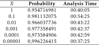
computes an estimatep0 ofp withconfidence1−δ, for which we have: P r(|p0−p|≤)≥1−δ. This procedure is based on the Chernoff-Hoeffding bound[24], which provides the minimum number of simulations required to ensure the desired confidence level.
The quantitative approach is used when there is no known approximation of the probability to evaluate, i.e. to obtain a first approximation. This method is useful when the goal of the analysis is to have an idea on how well the model behaves. On the contrary, the qualitative approach determines whether the probability is above a given threshold, with a high confidence and in a minimal number of simulations.
5. Timed OCL Constraints for SoS Requirements
The challenge in promoting the use of formal specifi-cation languages in an industrial setting is essentially to provide a good balance between expressiveness and usability. The SoS setting introduces further challenges for the need of specifying properties of the state of com-plex systems and architectures. For scalability reasons, monolithic verification approaches should be avoided in favor of compositional ones, such as those based on thetheory of contracts[25].
In this section we present the requirements language, called GCSL (Goals and Contracts Requirement Lan-guage). The full GCSL language specification, as well as the details of translation of the GCSL patterns into BLTL, can be retrieved in [26]. In this section we focus on providing a brief recap of the language and illustrate why it is appropriate to define SoS and CSs require-ments. We also discuss an explicit contribution of this paper to GCSL.
5.1. A Survey of GCSL
A GCSL contract is a pair of Assume/Guarantee assertions:
GCSL_Contract := hAssume,Guaranteei
denoting requirements on SoS and CSs inputs and outputs, respectively. Contracts allow us to decompose requirements and perform local or global verification on need [25].
Assertions are built upon GCSL natural-language patterns: we summarize in Figure 1 the principal patterns used in the DANSE project. GCSL pat-terns are inspired by and extend the Contract Spec-ification Language (CSL) patterns [27], developed in the SPEEDS European project. These natural-language based requirements have their formal seman-tics defined by translation into corresponding BLTL formulas, enabling the application of SMC. To sim-plify the specification of properties of complex systems and architectures, GCSL integrates the Object Con-straint Language (OCL) [28], a formal language used
8 EAI Endorsed Transactions
on
Industrial Networks and Intelligent Systems
to describe static properties of UML models. OCL is an important means to improve the expressiveness and usability of GCSL patterns. Using OCL we can describe properties about types of CS in the SoS architecture, while being independent of their actual number of instances and, thus, defining requirements that are adaptable to the natural evolution of the SoS, without the need of rewriting them. OCL allows us also to define algebraic constraints over Constituent Systems attributes. In summary, GCSL Patterns are able to express real-time constraints over complex portions of the entire SoS state.
To show the expressiveness of GCSL, let us consider the following simple example (based on Pattern 9 from Fig. 1):
SoS.its(CriticalComponent)→forAll(cc|
whenever
[cc.its(TempSensor)→exists(ts|ts.temp>cc.threshold) ]
occurs,
[cc.connected(CoolingFan)→exists(f|f.on) ]
occurs within[1 min,5 min] )
This architecture-abstract requirement says that if any CS of type CriticalComponent has one of its
TempSensor measuring at time t a temperature
that is higher than the threshold set by the specific CriticalComponent (the threshold may be different for distinct components) then one of the CoolingFan connected to that component should be switched on within the [t+1 min,t+5 min] time frame. This property does not depend on a concrete architecture or on the number and identity of the mentioned CSs. It can be used as a requirement for any SoS having an architecture that integrates the mentioned CSs types. Moreover, this requirement is still valid even if the SoS changes its architecture, either for intrinsic reconfiguration needs or for external design or re-configuration activity. Therefore, GSCL requirements are valid for the entire lifetime of the system and need not be reformulated at any architectural change.
The idea of mixing OCL and temporal logic originates from the need of specifying static and dynamic properties of object-based systems. In [29, 30] OCL has been extended with CTL and (finite) LTL, respectively, without support for real-time properties. The work in [31] is more similar to ours and it is based on ClockedLTL, a real-time extension of LTL. ClockedLTL is slightly more expressive than BLTL, because it allows unbounded temporal operators, whereas BLTL is decidable on a finite trace. On the contrary, BLTL does not include unbounded operators because SMC requires to decide a property on a given finite trace.
As mentioned previously, the introduction and use of patterns is motivated by infeasibility of direct use of BLTL, which is a very low level language. Indeed, commonly used properties may require the
nesting of several BLTL temporal operators, with the effect of increasing the risk of errors in requirements formulation and reducing their readability. Patterns provide a convenient way to represent frequently-occurring and well-identified property templates, while avoiding errors due to the complexity of the underlying logic. The methodology developed during the DANSE project prescribes to have a library of patterns [26] that captures the most relevant temporal constraints for the considered domain. So a pattern-library shall be considered as an important asset that is tailored to specific design needs.
Description of the patterns. In the rest of this section we are going to discuss a number of these pre-defined patterns. Clearly, as already discussed, the choice of the set of patterns is inevitably subjective and depends on the field of application as well as on the test case at hand. The expressiveness of BLTL, jointly with OCL, makes the patterns library easily extensible to cover future, domain-specific needs.
Figure 1 shows the most relevant GCSL patterns used in the DANSE project [26]. For every pattern, there is the corresponding BLTL translation that illustrates how temporally-bounded BLTL operators are used and how it can be complex to reason directly in terms of those operators. In all the following patterns, Ψ denotes an argument where an OCL property can be used to describe a state of the SoS. The keywords ‘occurs’ and ‘holds’ are used to indicate, respectively, that there is at least one real-time instant where the given property shall be satisfied or that in all real-time instants the given property shall be satisfied. Constants a,b and c
specify bounds of time intervals and are real-time values. The constant nis an integer value, whilee is a value from 0 to 100, denoting a percentage.
Pattern 1 can be used to specify a causal relation
between a condition Ψ1 (e.g. system activated) and a consequential condition Ψ2 that is activated by and stable since the originating condition (e.g. active indication light is on).
Pattern 2 can be used to specify a typical invariant
property, which express a bound on the set of states the system shall traverse under any condition (e.g. the value of control signal is always within a specified interval). In particular, the OCL property Ψ should be true at every real-time instant within simulation end timek.
Pattern 3 can be used to specify a causal relation
between Ψ1 and Ψ2 that happens only within an absolute time-frame ([a,b]). It is interesting to see how the next operator X≤a is used to push to the very
for some patterns (as we shall see in the following) the bounds of time intervals are offsets referred to a previously occurred conditionΨ.
Pattern4 can be used to specify that a conditionΨ1that is held continuously in the absolute time-frame ([a,b]) causes the conditionΨ2to occur at the end of the time-frame. For example, to specify the need for a minimum duration of a certain condition before being able to activate the consequent. Clearly, a longer duration will also cause activation.
Pattern5 can be used to specify that if a conditionΨ1 shall be held continuously in the absolute time-frame ([a,b]) then the two other conditionsΨ2 and Ψ3 shall happen contiguously in the same time-frame. This pattern supports the specification of the decomposition of an activity (expressed by Ψ1) into sub-activities (expressed by Ψ2 and Ψ3). Further decomposition can be specified by conjunction with other properties using the same pattern over the contained time-frame ([a,c]) or ([c,b]).
Pattern6 can be used to constrain the number of times
a condition Ψ can be active within an absolute time-frame. Its translation relies on the BLTL operator occ
and, even if it does not involve any temporal operator, it cannot be decided on a single state but it needs to be checked across the entire simulation trace.
Pattern7 can be used to specify a conditionΨ2 that is triggered by the number of times a conditionΨ is active within an absolute time-frame.
Patterns8and9 are not referred to an absolute
time-frame. They are used to specify a liveness property which is triggered by an initial conditionΨ1 occurring at time t and discharged by a following conditionΨ2 that occurs/holds within the interval [t+a, t+b] that is relative to the time t of occurrence of Ψ1. They are useful to express performance specifications such as, for example, the switching of an engine power-on buttpower-on at time t triggers the burning chamber temperature sensors to detect a temperature increase within t+ 10sec (minimal duration) and t+ 15sec
(maximal duration). Note that its translation into BLTL underpins a number of important assumptions. First, the pattern is verified on the entire simulation up to time k−b. This is needed because if a condition Ψ1 occurs atk−b, we need to have enough remaining time (actuallyb) to verify whether either it is discharged by a condition Ψ2 (making the pattern true) or not. As a consequence, a conditionΨ1 occurring after timek−b would not require any following discharging condition. Second, on the occurrence of a conditionΨ1the pattern requires a shift to timea(as close as possible, depending on the actual states produced by simulation) which is indicated by the next operator X≤a. From that point onwards, we can check for the occurrence of the conditionΨ2in the remaining interval usingF≤b−a.
Finally, Patterns10, 11, and 12 are typically used to
express reliability constraints, such as the availability of a system. The BLTL translation of these patterns relies on the #T imeandduroperators that we shall discuss in more details in the following. The first pattern requires that in every real-time instant t within the absolute time-frame ([a,b]) the amount of time a conditionΨ has been true is at leaste% oft. We use the operatordurto accumulate the overall time during whichΨ is true, and we compare the accumulated value with the required portion of the current simulation time, extracted with the operator #Time, at each simulation point. A typical example use of this property is the specification of the system up-time. This can be done by specifying a conditionΨ that captures the states of the system where there is either no fault or a number of faults against which the system has adequate countermeasures. The second pattern is slightly more permissive, allowing to violate the constraint at intermediate real-time instants, but requiring that, at the end of the absolute time-frame ([a,b]), the constraint is satisfied. Note that, in both cases, the lower bound a of the absolute time-frame ([a,b]) is used to ensure that there are no constraints in the initial system lifetime, where early failures may be expected and not critical. Finally, the last pattern is used when the constraint is applied from the beginning of simulation.
OCL constraints on architecture. We now turn our attention to the OCL part of GCSL and to how it helps us improve the expressiveness of the patterns and the adequacy to the SoS domain. Figure 2 shows a (simplified) portion of the grammar defining the OCL integration within the GCSL atomic properties (indicated by OCL-prop). Properties are constructed using usual boolean operators (◦) and basic arithmetic comparisons (./) between expressions. Attributes of Constituent Systems can occur in properties or expressions and can be accessed by using their Fully Qualified Name (FQN), which is essentially their path from the top of the SoS down through the containment hierarchy collecting Constituent Systems names (csName) and terminating with the attribute name (attribute), such asSoS.Sensor03.isOn.
The peculiarity of OCL propositions is the abil-ity to predicate properties of sets of yet unknown
(at requirements-definition time) Constituent Systems. These sets are left undetermined because the require-ments may apply to several variant architectures of the same SoS and the SoS architecture may evolve during the SoS life-cycle. Indeed, in [1] one of the five SoS-specific properties of a complex system is that the number and type of systems participating to a SoS may change over time. Ideally, the specifications of the system should remain independent of the number and type of CSs, which is exactly what OCL provides as a feature within GCSL. In order to support properties
10 EAI Endorsed Transactions
on
Industrial Networks and Intelligent Systems
ID Pattern (below,kis the simulation time anda < c < b≤k)
1 [Ψ1] occurs implies that [Ψ2] holds forever G≤−1(Ψ1→G≤−1(Ψ2))
2 [Ψ] holds G≤−1(Ψ)
3 [Ψ1] implies [Ψ2] holds during [a,b] X≤aG≤b−a(Ψ1→Ψ2)
4 [Ψ1] holds during [a,b] raises [Ψ2] (X≤aG≤b−a(Ψ1))→X≤b(Ψ2)
5 [Ψ1] holds during [a,b] implies [Ψ2] holds during [a,c] then [Ψ3] holds during [c,b] (X≤aG≤b−a(Ψ1))→(X≤aG≤c−a(Ψ2)∧X≤cG≤b−c(Ψ3))
6 [Ψ1] occurs at least (at most)ntimes during [a,b] occ(Ψ1,a,b)≥(≤)n
7 [Ψ1] occurs at least (at most)ntimes during [a,b] raises [Ψ2] occ(Ψ1, a, b)≥(≤)n→X≤bF≤−1(Ψ2) 8 whenever [Ψ1] occurs [Ψ2] holds during following [a,b] G≤−1(Ψ1→X≤aG≤b−a(Ψ2))
9 whenever [Ψ1] occurs [Ψ2] occurs within [a,b] G≤−1(Ψ1→X≤aF≤b−aΨ2)
10 always during [a,b], [Ψ] has been true at least [e] % of time G≤b(#Time< a∨dur(Ψ)≥(100e ∗#Time)) 11 at the end of [a,b] [Ψ] has been true at least [e] % of time X≤aF≤b(dur(Ψ)≥100e ∗(b−a))
12 at [b], [Ψ] has been true at least [e] % of time F≤b(dur(Ψ)≥100e ∗b)
Figure 1. GCSLPatterns and their BLTL translations, with Ψ,Ψ1,Ψ2∈OCL-prop,a, b∈R,e∈OCL-expr
OCL-prop ::= true|false|FQN|notOCL-prop|OCL-prop◦OCL-prop|OCL-expr./OCL-expr|
OCL-coll→forAll(var|OCL-prop[var])|OCL-coll→exists(var|OCL-prop[var])|
OCL-coll→empty()|OCL-coll→notempty()
OCL-expr ::= FQN|OCL-coll→sum()|OCL-coll→size()|. . .
OCL-coll ::= attribute|csName|its(type)|connected(type)|OCL-coll.OCL-coll
Figure 2. Simplified OCL fragment forGCSLAtomic Properties, with◦ ∈ {∧,∨,→,↔}and ./∈ {>,≥,=, <,≤}.
that are parametrized by the SoS architecture, GCSL provides the quantifiersforAllandexiststhat allow us to instantiate properties over finite collections ( OCL-coll) of Constituent Systems (thevarranges over these collections and occurs in the OCL-prop which is the scope of the quantifier). A corner case of quantification is provided by the set operators emptyand notempty
that simply return a truth value after testing the empti-ness of the collection.
It is interesting to discuss how collections ( OCL-coll) are specified, as it is a peculiarity of GCSL extending the standard OCL language. Standard OCL allows concatenating object names (here indicated as
csName) by the “.”-containment relation, until reaching an attribute. In GCSL we add (1) another (weak) containment operator (its) that allows to navigate the systems hierarchy by filtering on CS-type and (2) an operator (connected) that allows to navigate the neighborhood of a CS, again in terms of types. For example, the expression SoS.its(CriticalComponent) denotes the set of CSs of type CriticalComponent
and are contained in the system named SoS. The expression SoS.cc01.connected(CoolingFan) denotes the set of CSs of type CoolingFan that are connected to the critical component cc01, which is itself contained in the system named SoS. Quantifiers occur also in expressions (OCL-expr) and allow aggregating the values of (equally-typed) attributes. E.g. the simple expression (SoS.its(Sensor).temp→sum( ))/(SoS.its(Sensor)→size( ))
can be used to compute the average temperature in a SoS where the number of CS of type Sensor is unknown or time-dependent.
Architecture-dependent translation of OCL. Before conclud-ing this section, we should discuss how the translation of GCSL into BLTL is handled for OCL. Since BLTL does not interpret the OCL syntax (except for FQN), the translation from GCSL to BLTL requires the pre-liminary elimination of all the OCL operators (forAll,
exists, empty, notempty, sum, size, its, connected). This elimination step can be performed only once the SoS architecture is determined and it is valid for a fixed architecture state.
OCL operators can be nested and their elimination is performed by induction over the structure of the formula in an outside-in fashion. Conceptually, this can be done by applying the following algorithm:
1. resolution of the outermost OCL collections (that is, replacing a collection with afiniteset ofFQN), which eliminates ‘its’ and ‘connected’ operators,
2. elimination of the universal (existential) quanti-fiers, replaced by the corresponding conjunctions (disjunctions) of the instantiated scopes,
3. elimination of the remaining operators by replacement with corresponding Boolean or arithmetic expressions, and
Termination of the algorithm is trivially proved by considering that (i) the number of nested operators is always finite and strictly decreasing at every rewriting step, and (ii) that all the OCL collections contain finitely many elements that are defined by the current state of the architecture. Note that this translation needs be performed every time there is architecture state change. Therefore, the tool-chain dynamically evaluates the formula as the architecture changes. One needs to consider that translation may potentially introduce a combinatorial blow-up of the formula, which suggests the need of adopting an on-the fly evaluation algorithm. To illustrate the elimination of OCL operators on a concrete example, assume that the requirement considered previously is checked on the architecture in Figure 3. In that Figure, instances whose name start by “cc” are of type CriticalComponent, instances whose name start by “cf” are of type CoolingFan, and finally instances whose name start by “ts” are of type TempSensor. In this case, the collec-tionSoS.its(CriticalComponent) would be resolved into the set {SoS.cc01,SoS.cc02}. Then, the new outermost collections would be SoS.cc01.its(TempSensor),
SoS.cc01.connected(CoolingFan),
SoS.cc02.its(TempSensor), and
SoS.cc02.connected(CoolingFan). These are further resolved into the following sets: {SoS.cc01.ts01,
SoS.cc01.ts02}, {SoS.cc01.cf01}, {SoS.cc02.ts03}, and {SoS.cc02.cf01,SoS.cc02.cf02}, respectively.
As a consequence of the translation against the considered architecture, the formula would be:
whenever
[SoS.cc01.ts01.temp>SoS.cc01.threshold∨
SoS.cc01.ts02.temp>SoS.cc01.threshold]
occurs
[SoS.cf01.on]
occurs within[1 min,5 min]
∧
whenever
[SoS.cc02.ts03.temp>SoS.cc02.threshold]
occurs
[SoS.cf01.on∨SoS.cf02.on]
occurs within[1 min,5 min]
This elimination-based approach is justified by the fact that SoS development with architecture reconfiguration has, typically, a larger time-scale than the operational level of the CSs. So architecture snapshots can be individually analysed, while architectures alternatives are generated from generic architectural pattern.
After having illustrated the main features of GCSL and how they support the SoS specification and dynamic evolution challenges we discuss, in the following section, how to obtain a unique behavioural model of the SoS by integration of single and heterogeneous CSs behavioural models.
Figure 3. Architecture with connection (e.g.cc01−cf01) and
containment (e.g.cc01−ts01) relations.
6. Performing Statistical Model Checking
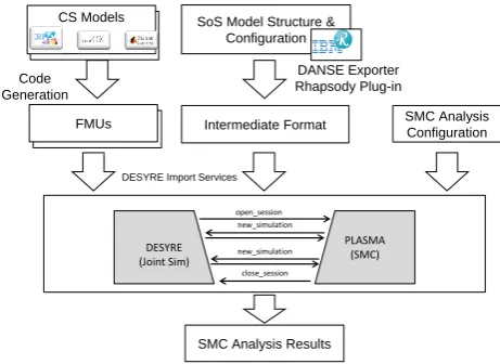
This Section describes the work-flow and its supporting tool-chain (see Figure 4) we have set-up to accomplish statistical model checking analysis on Systems of Systems models.
Our tool-chain has been adopted by the industry partners of the DANSE Project: CARMEQ, IBM, EADS, and Thalès. The core of our SMC tool-chain is composed of three main tools: IBM Rhapsody is the tool implementing the UPDM language to model SoS architectures, DESYRE [8–10] is the tool providing the joint simulation engine for SMC and PLASMA [5] is the tool providing the SMC analysis engine. Other modelling tools like Modelica and Simulink/Stateflow surround this core tool-chain to provide behavioural models in the form of FMUs.
6.1. SMC Analysis Workflow
Figure 4 shows our SMC analysis work-flow. The work-flow starts with two parallel branches. The topmost block of the left branch represents the parallel development of Constituent Systems’ models, each with its best-fitting modelling tool as described in Section 2.1. The topmost block of the right branch represents
DESYRE (Joint Sim)
PLASMA (SMC)
open_session new_simulation
new_simulation close_session
SMC Analysis Configuration
SMC Analysis Results FMUs
CS Models
SoS Model Structure & Configuration
Intermediate Format FMUs
CS Models
Code Generation
DANSE Exporter Rhapsody Plug-in
DESYRE Import Services
Figure 4. SMC Analysis Workflow.
12
EAI Endorsed Transactions on
Industrial Networks and Intelligent Systems
the development of the SoS architecture in UPDM as described in Section 2.2. Once each CS model gets ready for joint-simulation and SMC analysis, it is exported from its modelling tool into the FMI-compliant format. This step is represented by blocks named “FMUs” in the left branch of Figure 4. On the right branch, when the UPDM blocks in the SoS architecture are 1) in synch with their corresponding CSs models (e.g. same interfaces) and 2) correctly interconnected, our Rhapsody exporter plug-in can be invoked to translate the UPDM model into a form that DESYRE can use to run joint-simulation. At this point of the work-flow all the information needed to run the statistical model checking analysis is available and to launch the SMC analysis the user has to provide a proper SMC analysis configuration.
6.2. The SMC Workflow from the User Perspective
IBM Rhapsody. IBM Rational Rhapsody [32] is a model-based system engineering environment implementing industry-standard languages such as UML, SysML and UPDM. Referring to Figure 4, IBM Rhapsody represents the starting point of the SMC analysis work-flow. The
Figure 5. DANSE Profiles and Stereotypes implemented in IBM
Rhapsody.
DANSE Exporter Rhapsody Plug-in
Execution
Figure 6. Export to DESYRE of IBM Rhapsody Model
Representing the SoS Architecture.
SoS architecture is specified within this tool by using the UPDM industry-standard language, conveniently extended to meet SMC analysis specification needs. Figure 5 shows how the UPDM extensions described in Section 2 have been implemented in IBM Rhapsody. At this point, the user will rely on the profiles to model the architecture of the SoS. This includes attaching GCSL contracts to the Constituent Systems and/or to the whole SoS.
During DANSE Project IBM has extended the Rhapsody tool to generate FMI 1.0 compliant FMUs from most of UPDM behavioural diagrams, thus making it join the pool of those candidate modelling and simulation tools able to export CS models for our SMC analysis purposes. In that context, the user can rely on our profiles for describing stochastic behaviors.
Exporting information for SMC. IBM Rational Rhapsody provides a Java API set for integration with external tools. We developed a Java Exporter Plug-in to translate information from the UPDM SoS architecture model, along with all the information related to SMC analysis i.e. GCSL requirements, FMU names and URIs, and traceability settings to a format intelligible by DE-SYRE, the joint simulation engine. Our Exporter Plug-in Plug-integrates Plug-into Rhapsody as an UPDM extension profile («DANSEExporterPlugIn» profile in Figure 5). Once invoked from the IBM Rhapsody “Tools” menu our Exporter recursively parses both the UPDM Block Definition Diagram and the Internal Block Diagram to translate all the information needed to perform SMC analysis into the DESYRE internal representation format (XMI). Figure 6 shows how the user exports the Rhapsody UPDM SoS model in the intermediate format compliant with the format expected by DESYRE.
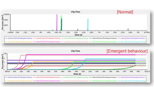
corresponding FMUs. At this point the user can run a simulation and graphically plot the evolution of some selected variables, as shown in 11.
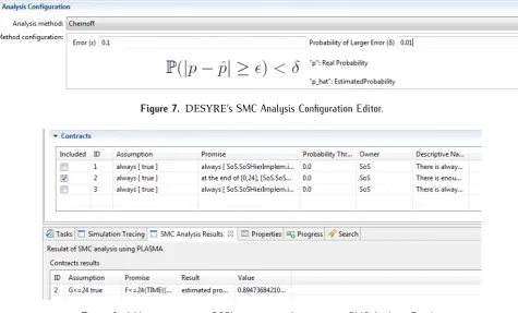
To run a DANSE statistical model checking analysis the user creates a statistical model checking config-uration in DESYRE. Figure 7 shows DESYRE’s SMC Analysis Configuration Editor. From the editor the user selects one SMC Analysis Method out of the ones pro-vided by PLASMA. Figure 7 shows that the Chernoff method has been selected. According to the selected analysis method the editor prompts the associated Anal-ysis Configuration frame to configure the parameters of the chosen algorithm. The user also specifies the simulation time of each SMC simulation run. GCSL contracts specified in the IBM Rhapsody UPDM model are available in the DESYRE intermediate representa-tion and can be imported into the SMC configurarepresenta-tion editor. In this case the user might not be interested in validating all the imported GCSL contracts through the SMC analysis she/he is configuring. To address this need we decided to make the imported GCSL contracts selectable by means of check-boxes. Such check-boxes are visible in Figure 8. The user can also directly write GCSL contracts from the GUI, or edit the ones imported from the UPDM description. To this end, the user can specify the new GCSL contract in its three components:
Assumption, Promise and Owner, the latter being the model element to which the GCSL contract predicates on. When the configuration is completed, the user can launch the SMC analysis campaign. After the SMC anal-ysis has terminated the user selects the SMC Analysis Results view, that appears as shown in Figure 8. SMC analysis results are displayed per GCSL requirement as shown in the bottom-right corner of Figure 8. On the figure, only one formula was evaluated, and its proba-bility to hold was evaluated to approximately 87%.
PLASMA. PLASMA is a tool for performing SMC analysis. Contrary to existing tools, PLASMA offers a modular architecture which allows plugging new simulators and new input languages on demand. This architecture has been exploited to verify systems and requirements from various languages/specific domains such as systems biology [33], a train station [34], or an autonomous robot [35].
The core of PLASMA is thus a set of SMC algorithms, which includes those presented in Subsection 4.2 as well as more complex ones [5]. This core is completed by two types of plug-ins, that are controlled by the SMC algorithm. First, the simulator plug-ins which implements an interface between PLASMA and a dedicated simulator to produce traces from a dedicated input language on demand. Second, there is a checker plug-ins that verify whether a finite trace satisfy a property.
For the purpose of this paper we extended the facilities of PLASMA as follows. First, we built a new plug-in between PLASMA and DESYRE in order to produce traces from FMI-FMU model. Second, we used the BLTL checker plug-in that we enrich with the two new primitivesdurand #T imein order to monitor those traces and report the answer to the SMC algorithm. As a last implementation effort, we also implemented a compiler from GCSL to BLTL.
Interaction between PLASMA and DESYRE. Once the user launches the analysis, DESYRE translates the GCSL properties to BLTL, as described in Section 5. It then invokes PLASMA and transmits the list of properties to check, as well as the algorithm and parameters to use. PLASMA then requests DESYRE to start the first execution. The execution is controlled step-by-step by PLASMA. At each step DESYRE provides a new snapshot of the system state, by giving the current value of every observed port in the architecture. A detailed description of the interaction between PLASMA and DESYRE is provided in [3].
7. A Case Study
This section illustrates the application of our technol-ogy to a concept alignment example that was defined for the DANSE Project. This case study has the partic-ularity to embed all the difficulties of the case stud-ies proposed by EADS, THALES, and CARMEQ that, for confidentiality reasons, cannot be described in this paper.
7.1. Modeling
We modeled an emergency response SoS for a city fire scenario in UPDM. The city is partitioned into 10 districts, and we focus on a few fire-fighting constituent systems (CS). We consider the following CSs: the Fire Head Quarter (FireHQ), the Fire Stations, the Fire Fighting Cars and the Fire Men. The behavior of the CSs has been modeled in several FMI-compliant authoring tools. For example, the FireMan has been modeled in OpenModelica (as shown in Figure 9) which is an open-source multi-domain modeling tool based on the Modelica language. Other CSs have been modeled using Rhapsody state-charts. The CSs rely on the new UPDM profile to include probabilistic behavior. For instance, each District models occurrences of fires by randomly choosing the time before the next fire according to an exponential distribution. The time before a fire is reported to the head quarter is also randomly chosen. We remind the reader that the objective of this work is not to learn the probability distribution itself (this has to be done via observations), but rather to show that it is conceptually possible to incorporate such information within the model.
14
EAI Endorsed Transactions on
Industrial Networks and Intelligent Systems