Support for End-to-End Response-Time and Delay
Analysis in the Industrial Tool Suite: Issues,
Experiences and a Case Study
?Saad Mubeen1, Jukka M ¨aki-Turja1,2, and Mikael Sj ¨odin1
1 M ¨alardalen Real-Time Research Centre (MRTC), M ¨alardalen University, Sweden 2
Arcticus Systems, J ¨arf ¨alla, Sweden
{saad.mubeen, jukka.maki-turja, mikael.sjodin}@mdh.se
Abstract. In this paper we discuss the implementation of the state-of-the-art end-to-end response-time and delay analysis as two individual plug-ins for the existing industrial tool suite Rubus-ICE. The tool suite is used for the development of software for vehicular embedded systems by several international companies. We describe and solve the problems encoun-tered and highlight the experiences gained during the process of imple-mentation, integration and evaluation of the analysis plug-ins. Finally, we provide a proof of concept by modeling the automotive-application case study with the existing industrial model (the Rubus Component Model), and analyzing it with the implemented analysis plug-ins.
Keywords:real-time systems, response-time analysis, end-to-end timing analysis, component-based development, distributed embedded systems.
1.
Introduction
Often, an embedded system needs to interact and communicate with its envi-ronment in a timely manner, i.e., the embedded system is a real-time system. For such a system, the desired and correct output is one which is logically correct as well as delivered within a specified time. The safety-critical nature of many real-time systems requires evidence that the actions by them will be provided in a timely manner, i.e., each action will be taken at a time that is ap-propriate to the environment of the system. Therefore, it is important to make accurate predictions of the timing behavior of these systems.
In order to provide evidence that each action in the system will meet its deadline,a priorianalysis techniques such as schedulability analysis have been developed by the research community. Response Time Analysis (RTA) [17, 45] is one of the methods to check the schedulability of a system. It calculates upper bounds on the response times of tasks or messages in a real-time system or a network respectively. Holistic Response-Time Analysis (HRTA) [48, 47, 42]
?
is an academic well established schedulability analysis technique to calculate upper bounds on the response times of task chains that may be distributed over several nodes in a Distributed Real-time Embedded (DRE) system.
A task chain is a sequence of more than one task in which every task (except first) receives a trigger, data or both from its predecessor. One way to classify these chains is as trigger and data. In trigger chains, there is only one triggering source (e.g, event, clock or interrupt) that activates the first task. The rest of the tasks are activated by their predecessors. In data chains, tasks are activated independent of each other, often with distinct periods. Each task (except the first) in these chains receives data from its predecessor. The first task in a data chain may receive data from the peripheral devices and interfaces, e.g., signals from the sensors or messages from the network interfaces. The end-to-end timing requirements on trigger chains are different from those on data chains. If a system is modeled with trigger chains only, it is called a single-rate system. On the other hand, if the system contains at least one data chain with different clocks then the system is said to be multi-rate.
The end-to-end delays should also be computed along with the holistic re-sponse times to predict complete timing behavior of multi-rate real-time systems [21]. For this purpose, the research community has developed the End-to-End3
Delay Analysis (E2EDA). In [21], the authors have a view that almost all auto-motive embedded systems are multi-rate systems. The industrial tools used for the development of these systems should be equipped with the state-of-the-art timing analysis.
A tool chain for the industrial development of component-based DRE sys-tems consists of a number of tools such as designer, compiler, builder, debug-ger, simulator, etc. Often, a tool chain may comprise of tools that are developed by different tool vendors. The implementation of state-of-the-art complex real-time analysis techniques such as RTA, HRTA and E2EDA in such a tool chain is non-trivial because there are several challenges that are encountered apart from merely coding and testing the analysis algorithms. These challenges and corresponding solutions that we propose are central to this paper.
Goals and Contributions. In this paper4, we discuss the implementation of HRTA and E2EDA as two individual plug-ins in the existing industrial tool suite Rubus-ICE (Integrated Component development Environment) [1]. Our goal is to transfer the state-of-the-art real-time analysis results, i.e., HRTA and E2EDA to the existing tools for the industrial use. We discuss and solve the problems encountered, solutions proposed and experiences gained during the implemen-tation, integration and evaluation of the plug-ins. We also provide a proof of con-cept by conducting the automotive-application case study. These new plug-ins support complete end-to-end timing analysis of DRE systems. Thus, the scope and usability of Rubus tools has widened with the addition of these plug-ins.
3
The terms “holistic” and “end-to-end” mean the same thing. In order to be consistent with the previous work and naming conventions used in the existing industrial tools, we will use “holistic” with response-times and “end-to-end” with delays.
4
Paper Layout. Section 2 presents the background and related work. Section 3 discusses the end-to-end timing requirements and the implemented analysis. Section 4 describes the challenges encountered, solutions proposed and ex-periences gained during the implementation and integration of the plug-ins. In Section 5, we present a case study by modeling and analyzing the automotive DRE application. Section 6 concludes the paper and presents the future work.
2.
Background and Related Work
2.1. The Rubus Concept
Rubus is a collection of methods and tools for model- and component-based de-velopment of dependable embedded real-time systems. Rubus is developed by Arcticus Systems [1] in close collaboration with several academic and industrial partners. Rubus is today mainly used for development of control functionality in vehicles by several international companies [2, 13, 7, 5]. The Rubus concept is based around the Rubus Component Model (RCM) [27] and its development environment Rubus-ICE, which includes modeling tools, code generators, anal-ysis tools and run-time infrastructure. The overall goal of Rubus is to be ag-gressively resource efficient and to provide means for developing predictable and analyzable control functions in resource-constrained embedded systems.
RCM expresses the infrastructure for software functions, i.e., the interaction between them in terms of data and control flow separately. The control flow is expressed by triggering objects such as internal periodic clocks, interrupts and events. In RCM, the basic component is called Software Circuit (SWC). Its execution semantics are: upon triggering, read data on datain-ports; execute the function; write data on dataout-ports; and activate the output trigger.
RCM separates the control flow from the data flow among SWCs within a node. Thus, explicit synchronization and data access are visible at the modeling level. One important principle in RCM is to separate functional code and infras-tructure implementing the execution model. RCM facilitates analysis and reuse of components in different contexts (SWC has no knowledge how it connects to other components). The component model has the possibility to encapsulate SWCs into software assemblies enabling the designer to construct the system at different hierarchical levels. Recently, we extended RCM for the development of DRE systems by introducing new components [30, 39, 33]. A detailed com-parison of RCM with several component models is presented in [39].
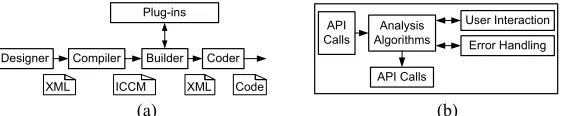
Fig. 1(a) depicts the sequence of main steps followed in Rubus-ICE from modeling of an application to the generation of code. An application is modeled in the Rubus Designer tool. Then the compiler compiles the design model into the Intermediate Compiled Component Model (ICCM). After that the builder tool sequentially runs a set of plug-ins. Finally, the coder tool generates the code.
2.2. The Rubus Analysis Framework
require-ments from a generated event and an arbitrary output trigger along the trig-ger chain. For this purpose, the designer has to express real-time properties of SWCs, such as worst-case execution times and stack usage. The scheduler will take these real-time constraints into consideration when producing a sched-ule. For event-triggered tasks, response-time calculations are performed and compared to the requirements. The analysis supported by the model includes response time analysis and shared stack analysis.
2.3. Plug-in Framework in Rubus-ICE
The plug-in framework in Rubus-ICE [26] facilitates the implementation of re-search results in isolation (without needing Rubus tools) and their integration as add-on plug-ins (binaries or source code) with the Rubus-ICE. A plug-in is interfaced with the builder tool as shown in Fig. 1(a). The plug-ins are exe-cuted sequentially which means that the next plug-in can execute only when the previous plug-in has run to completion. Hence, each plug-in reads required attributes as inputs, runs to completion and finally writes the results to the ICCM file. The Application Programming Interface (API) defines the services required and provided by a plug-in. Each plug-in specifies the supported system model, required inputs, provided outputs, error handling mechanisms and a user inter-face. Fig. 1(b) shows the conceptual organization of a plug-in in the Rubus-ICE.
τB τC τD
5 10 15 20 25
τC
0 30
τA
5 10 15 20 25
0 30
5 10 15 20 25
0 30
LIFO LILO (Data Age) FIFO (Data Reaction)
FILO
(b) τA
5 10 15 20 25
0 30
5 10 15 20 25
0 30
τB
Impossible Timed Path
5 10 15 20 25
0 30
τC
5 10 15 20 25
0 30
τD
5 10 15 20 25
τE
0 30
(a)
(a) Node A
ISWC_A SWC_A OSWC_A
Node B
ISWC_B SWC_B OSWC_B
Option 2 (b) m2 Node B τSWC_B τOSWC_B τISWC_B Node A τSWC_A τISWC_A m1 τOSWC_A Node A τA Option 1
m2 m1
Node B τB API Calls Analysis Algorithms User Interaction Error Handling API Calls
Designer Compiler Builder Coder
XML XML
Plug-ins
ICCM Code
(b) (a)
Fig. 1.Sequence of steps from design to code generation in Rubus-ICE
2.4. Response-Time Analysis
RTA of Tasks in a Node. Liu and Layland [28] provided theoretical foundation for analysis of fixed-priority scheduled systems. Joseph and Pandya published the first RTA [25] for the simple task model presented in [28]. Subsequently, it has been applied and extended in a number of ways by the research community. RTA applies to systems where tasks are scheduled with respect to their priori-ties and which is the predominant scheduling technique used in real-time oper-ating systems [40]. Tindell [47] developed the schedulability analysis for tasks with offsets for fixed-priority systems. It was extended by Palencia and Gon-zalez Harbour [42]. Later, M ¨aki-Turja and Nolin [29] reduced pessimism from RTA developed in [47, 42] and presented a tighter RTA for tasks with offsets by accurately modeling inter-task interference. We implemented tighter version of RTA of tasks with offsets [29] as part of the HRTA and E2EDA.
CAN which has served as a basis for many research projects. Later on, this analysis was revisited and revised by Davis et al. [19]. The analysis in [49, 19] assumes that all CAN device drivers implement priority-based queues. In [20] Davis et al. pointed out that this assumption may become invalid when some nodes in a CAN network implement FIFO queues. Hence, they extended the analysis of CAN with FIFO queues as well. In this work, the message deadlines are assumed to be smaller than or equal to the corresponding periods. In [18], Davis et al. lifted this assumption by supporting the analysis of CAN messages with arbitrary deadlines. Furthermore, they extended their work to support RTA of CAN for FIFO and work-conserving queues.
However, the existing analysis does not support mixed messages which are implemented by several high-level protocols for CAN. In [32, 36, 31], Mubeen et al. extended the existing analysis to support RTA of mixed messages in the CAN network where some nodes use FIFO queues while others use priority queues. Later on, Mubeen et al. [38] extended the existing analysis for CAN to support mixed messages that are scheduled with offsets in the controllers that implement priority-ordered queues. In this work we will consider all of the above analyses as part of the end-to-end response-time and delay analysis.
Holistic RTA. The holistic response-time analysis calculates the response times of event chains that are distributed over several nodes (also called dis-tributed transactions) in a DRE system. It combines the analysis of nodes (uni-processors) and networks. In this paper, we consider the end-to-end timing model that corresponds to the holistic schedulability analysis for DRE systems [48]. In [34], we discussed our preliminary findings about implementation issues that are encountered when HRTA is transferred to the industrial tools.
End-to-end Delay Analysis. Stappert et al. [46] formally described end-to-end timing constrains for multi-rate systems in the automotive domain. In [21], Feiertag et al. presented a framework (developed in TIMMO project [16]) for the computation of end-to-end delays for multi-rate automotive embedded systems. Furthermore, they emphasized on the importance of two end-to-end latency se-mantics, i.e., “maximum age of data” and “first reaction” in control systems and body electronics domains respectively. A scalable technique, based on model checking, for the computation of end-to-end latencies is described in [43]. In this work, we will implement the end-to-end delay analysis of [21].
2.5. Tools for End-to-end Timing Analysis of DRE Systems
Network (LIN) and CAN. It also supports end-to-end timing analysis of a system with more than one network. It implements RTA of CAN presented in [49].
SymTA/S [23] is a tool for model-based timing analysis and optimization. It implements several real-time analysis techniques for single-node, multiproces-sor and distributed systems. It supports RTA of software functions, RTA of bus messages and end-to-end timing analysis of both single-rate and multi-rate sys-tems. It is also integrated with the UML development environment to provide a timing analysis support for the applications modeled with UML [22].
Vector [11] is a tools provider for the development of networked electronic systems in the automotive and related domains. In the Vector tool family, CANoe [3] is a tool for the development, testing and analysis of ECU (Electronic Control Units) networks and individual ECUs. It supports various protocols for network communication including CAN, LIN, MOST, Flexray, Ethernet and J1708. Net-work Designer CAN is another tool by Vector that is used to design the architec-ture and perform timing analysis of CAN network. RAPID RMA [8] implements several scheduling schemes and supports end-to-end analysis for single- and multiple-node real-time systems. It also allows real-time analysis support for the systems modeled with Real-Time CORBA [44].
The Rubus-ICE tool suite allows a developer to specify timing information and perform the HRTA and E2EDA at the modeling phase during component-based development of DRE systems. To the best of our knowledge, Rubus-ICE is the first and only tool suite that implements RTA of mixed messages in CAN [32], RTA of mixed messages with offsets [38] and a tighter version of offset-based RTA algorithm [29] as part of the HRTA and E2EDA .
3.
End-to-end Timing Requirements and Implemented
Analysis in Rubus-ICE
3.1. End-to-end timing requirements in trigger chains
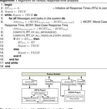
A real-time system (single-node or distributed) can be modeled with trigger chains (see Fig.2(a)), data chains (see Fig.2(b)) or a combination of both. The end-to-end timing requirements on trigger chains are different from those on data chains. If the system is modeled with trigger chains then the end-to-end deadline requirements are placed on the holistic response times.
An example of a trigger chain that consists of three components is shown in Fig. 2(a). Assume that each component corresponds to a task at run-time. When taskτSWC A finishes its execution, it triggersτSWC B. Similarly,τSWC C
3.2. End-to-end timing requirements in data chains
As compared to the systems which are modeled with trigger chains, merely computing the holistic response times and comparing them with the end-to-end deadlines is not sufficient to predict the complete timing behavior of multi-rate real-time systems which are modeled with data chains. There may be over-and under-sampling in such systems because the individual tasks are activated by independent clocks, often with different periods. Since data is transferred among tasks and messages within a data chain by means of asynchronous buffers, there exist different semantics of end-to-end delay in a data chain. These buffers are often of a non-consuming type which means the data stays in the buffer after it is read by the reader task. Moreover, the data in the buffer can be overwritten by the writer task with new values before the previous value was read by the reader task. Therefore, some input values in the data buffers can be overwritten by new values, and hence the effect of the old input values may never propagate to the output of a data chain. Further, there may be several duplicates of the output of a data chain corresponding to a particular input.
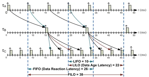
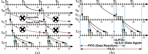
The end-to-end timing requirements in multi-rate real-time systems, espe-cially in the automotive domain, are placed on the first reaction to the input and age of the data at the output [21]. The end-to-end delay in a data chain refers to the time elapsed between the arrival of a signal at the first task and production of corresponding output signal by the last task in the chain (provided the infor-mation corresponding to the input has traversed the chain from first to last task) [43]. In a single-rate real-time system that contains only trigger chains, tasks in a chain are not activated by independent events, in fact, there is only one ac-tivating event in the chain. Hence, the holistic response times and end-to-end delays will have equal values. On the other hand, these values are not the same in multi-rate real-time systems that are modeled with data chains. Therefore, a complete analysis of a real-time system modeled with data chains requires the calculation of not only holistic response times but also end-to-end delays. Examples. A multi-rate real-time system modeled with three SWCs in RCM is shown in Fig. 2(b). These SWCs are activated by independent clocks with different periods, i.e., 8ms, 16ms and 4ms respectively. SWC Areads the in-put signals from the sensors whileSWC C produces the output signals for the actuators. Assume that each SWC will be allocated to an individual task by the run-time environment generator. Also assume that WCET of each task is 1ms. The time line corresponding to the run-time execution of the three tasks (corresponding to three SWCs), depicted in Fig. 3, shows multiple outputs cor-responding to a single input. The four end-to-end delays are also identified.
Last In First Out (LIFO). This delay is equal to the time elapsed between
the current non-overwritten release of task τA (input of the data chain) and
corresponding first response of taskτC(output of the data chain).
Last In Last Out (LILO). This delay is equal to the time elapsed between the
current non-overwritten release of taskτAand corresponding last response of
task τC. This delay is identified as “Data Age”5 in [21]. Data age specifies the
5
longest time data is allowed to age from production by the initiator until the data is delivered to the terminator. This delay finds its importance in control applications where the interest lies in the freshness of the produced data. For a data chain in a control system that initiates with a sensor input and terminates by producing an actuation signal, it is very important to ensure that the actuator signal does not exceed a maximum age [21]. Generally speaking, we consider the last non-overwritten input that actually propagates through the data chain towards the output in the case of both LIFO and LILO delays.
8 ms 16 ms 4 ms
SWC_A SWC_B SWC_C
Sensor Input Data sink
10 ms SWC_A SWC_B SWC_C
Sensor Input Data sink
(a) (b)
Fig. 2.RCM model of (a) trigger chain (b) data chain in a single-node real-time system
/,)2
IJ&
/,/2'DWD$JH/DWHQF\ ),)2'DWD5HDFWLRQ/DWHQF\
),/2 IJ%
IJ$
t (ms)
t (ms)
t (ms)
Fig. 3.End-to-end delays for a data chain in a real-time system
First In First Out (FIFO). This delay is equal to the time elapsed between the
previous non-overwritten release of taskτAand first response of taskτC
corre-sponding to the current non-overwritten release of taskτA. Assume that a new
value of the input is available in the input buffer of taskτA“just after” the release
of the second instance of taskτA(at time 8ms). Hence, the second instance of
task τA “just misses” the read of the new value from its input buffer. This new
value has to wait for the next instance of taskτA to travel towards the output
of the data chain. Therefore, the new value will be read by the third and forth instances of taskτA. The first output corresponding to the new value (arriving
just after 8ms) will appear at the output of the chain at 34ms. This will result in the FIFO delay of 26ms as shown in Fig. 3. This phenomenon is more obvious in the case of distributed embedded systems where a task in the receiving node may just miss to read fresh signals from a message that is received from the network. This delay is identified as “first reaction or Data Reaction”6in [21]. It is equal to the longest allowed reaction time for data produced by the initiator to be delivered to the terminator. It finds its importance in button-to-reaction appli-cations in body electronics domain where first reaction to input is important.
6
First In Last Out (FILO). It is equal to the time elapsed between the previous non-overwritten release of taskτA and last response of taskτCcorresponding
to current non-overwritten release of taskτA. The reasoning about “just missing”
a fresh input (in the case of FIFO delay) is also applicable in this case.
The modeling of data chains and the definition of their end-to-end delays in distributed real-time systems is done in a similar fashion.
3.3. Implemented Holistic Response-Time Analysis
In order to analyze tasks in each node, we implement RTA of tasks with offsets developed by [47, 42] and improved by [29]. We implement the network RTA that supports the analysis of CAN and its high-level protocols. It is based on the following RTA profiles for CAN: (1) RTA of CAN [49, 19]; (2) RTA of CAN for mixed messages [32]; (3) RTA of CAN for mixed messages with offsets [38] (The analysis of this profile is implemented as a standalone analyzer).
The pseudocode of HRTA algorithm is shown in Algorithm 1. The HRTA al-gorithm iteratively runs the alal-gorithms for node and network analyses. In the first step, release jitter of all messages and tasks in the system is assumed to be zero. The response times of all messages in the network and all tasks in each node are computed. In the second step attribute inheritance is carried out. This means that each message inherits a release jitter equal to the difference be-tween the worst- and best-case response times of its sender task (computed in the first step). Similarly, each task that receives the message inherits a release jitter equal to the difference between the worst- and best-case response times of the message (computed in the first step). In the third step, response times of all messages and tasks are computed again. The newly computed response times are compared with the response times previously computed in the first step. The analysis terminates if the values are equal otherwise these steps are repeated. The conceptual view of HRTA plug-in is shown in Fig. 4.
3.4. Implemented End-to-end Delay Analysis
We implemented the end-to-end delay analysis that is derived in [21] as the E2EDA plug-in for Rubus-ICE. This analysis implicitly requires the calculation of response times of individual tasks, messages and holistic response times of task chains. For example, the calculation of four end-to-end delays for the multi-rate real-time system shown in Fig. 2(b) requires the response time of the task
τC(corresponding to the componentSWC C) and the activation times of tasks τAandτC. Since, the HRTA plug-in is able to calculate response times of tasks,
Algorithm 1Algorithm for holistic response-time analysis 1: begin
2: RTPrev←0 .Initialize all Response Times (RTs) to zero
3: Repeat←TRUE
4: whileRepeat =TRUE do
5: for allMessages and tasks in the systemdo
6: JitterMsg←(WCRTSender task−BCRTSender task) .WCRT: Worst-Case
Response Time, BCRT: Best-Case Response Time 7: JitterReceiver task←(WCRTMsg−BCRTMsg)
8: COMPUTERT OF ALL MESSAGES()
9: COMPUTERT OF ALL TASKS IN EVERY NODE()
10: ifRT>RTPrevthen
11: RTPrev←RT
12: Repeat ←TRUE
13: else
14: Repeat ←FALSE
15: end if
16: end for
17: end while
18: end
Rubus Builder
End-to-end timing information
Analysis Results
HRTA Plug-in
Algorithms for RTA of tasks in a node
Algorithms for RTA network messages
HRTA Algorithm E2EDA Plug-in
Algorithm for end-to-end delay analysis End-to-end timing information
Analysis Results
Fig. 4.Conceptual view of the E2EDA plug-in in Rubus-ICE
4.
Encountered Problems, Solutions and Experiences
In this section we discuss several problems encountered during the process of implementation and integration of HRTA and E2EDA as plug-ins for the Rubus-ICE tool suite. We also present our solution to each individual problem.
4.1. Extraction of Unambiguous Timing Information
Algorithm 2Algorithm for end-to-end delay analysis 1: begin
2: GET RT OF ALL TASKS MESSAGES TASK CHAINS() .Get the analysis results from the HRTA plug-in
3: FIND ALL VALID TIMEDPATHS().Timed Path (TP) is a sequence of task instances from input to output. A TP is valid if information flow among tasks is possible [21], e.g., [τA(1stinstance),τB(1stinstance),τC(5thinstance)] in Fig. 3 is a valid TP. On the
other hand, TP [τA(1stinstance),τB(1stinstance),τC(1stinstance)] in Fig. 3 is invalid
because information cannot flow betweenτB(1stinstance) andτC(1stinstance)
4: procedureCOMPUTEFF DELAY(FF TP)
5: FF delay =αn(instance) +δn(instance) -α1(instance) . αn(instance): Activation
time of the corresponding instance of the nthtask in timed path FF TP
. δn(instance): Response time of the corresponding instance of the nthtask in
timed path FF TP 6: returnFF delay 7: end procedure
.The above mentioned procedure calculates FFDelayonly. [21] should be
referred for the calculation of the rest of the delays 8: for allDelay constraints specified in the systemdo
9: FFDelay ←0,FLDelay←0,LFDelay ←0,LLDelay ←0 .Initialize all delays
10: COMPUTE ALL REACHABLE TIMED PATHS() .All those paths from
input to output in which the changes in input actually travel towards the output, e.g., [τA(2ndinstance),τB(1stinstance),τC(5thinstance)] in Fig. 3
11: FF TPcount←GET ALL FF TPS() .TP: Timed Path, FF: First to First
12: FL TPcount ←GET ALL FL TPS() .FL: First to Last
13: LF TPcount ←GET ALL LF TPS() .LF: Last to First
14: LL TPcount ←GET ALLLL TPS() .LL: Last to Last
15: fori:=1doFF TPcount
16: ifCOMPUTE FFDELAY(i)>FFDelaythen
17: FFDelay ←COMPUTE FFDELAY()
18: end if
19: end for
20: fori:=1doFL TPcount
21: ifCOMPUTE FLDELAY(i)>FLDelaythen
22: FLDelay←COMPUTEFL DELAY()
23: end if
24: end for
25: fori:=1doLF TPcount
26: ifCOMPUTE LFDELAY(i)>LFDelaythen
27: LFDelay←COMPUTELF DELAY()
28: end if
29: end for
30: fori:=1doLL TPcount
31: ifCOMPUTE LLDELAY(i)>LLDelay then
32: LLDelay ←COMPUTELLDELAY()
33: end if
34: end for
35: end for
analysis models are often build upon different meta-models [22]. Moreover, the design model can contain redundant timing information. Hence, it is not trivial to extract unambiguous timing information for HRTA and E2EDA. The timing information (to be extracted) can be divided into two categories.
Extraction of Timing Information Corresponding to User Inputs. The first category corresponds to the timing attributes of tasks and network messages that are provided in the modeled application by the user. These timing at-tributes include Worst Case Execution Times (WCETs), periods, minimum up-date times, offsets, priorities, deadlines, blocking times, precedence relations in task chains, jitters, etc. In [33], we identified all the timing attributes of nodes, networks, transactions, tasks and messages that are required by the HRTA. Extraction of Timing Information from the Modeled Application. The sec-ond category correspsec-onds to the timing attributes that are not directly provided by the user but they must be extracted from the modeled application. For ex-ample, message period (in periodic transmission) or message inhibit time (in sporadic transmission) is often not specified by the user. These attributes must be extracted from the modeled application because they are required by the RTA of network communication. In fact, a message inherits the period or inhibit time from the task that queues it. Thus, we assign period or inhibit time to the message which is equal to the period or inhibit time of its sender.
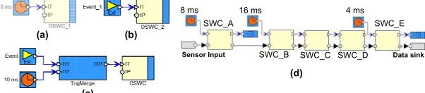
However, the extraction of message timing attributes becomes complex when the sender task has both periodic and sporadic activation patterns. In this case, not only the timing attributes of a message have to be extracted but also the transmission type of the message has to be identified. This problem can be visualized in the example shown in Fig. 5. It should be noted that the Out Soft-ware Circuit (OSWC), shown in the figure, is one of the network interface com-ponents in RCM that sends a message to the network. Similarly, In Software Circuit (ISWC) receives a message from the network [39].
In Fig. 5(a), the sender task is activated by a clock, and hence the corre-sponding message is periodic. Similarly, the correcorre-sponding message is spo-radic in Fig. 5(b) because the sender task is activated by an event. However, the sender task in Fig. 5(c) is triggered by both a clock and an event. Here the relationship between two triggering sources is important. If there exists a de-pendency relation between them as in the case of mixed transmission in the CANopen protocol [4] and AUTOSAR communication [9] then such message will be treated as a special type of sporadic message. If triggering sources are independent of each other (e.g., in the HCAN protocol [15]), the corresponding message will be considered a mixed message [32, 36]. If there are periodic and sporadic messages in the application, the HRTA plug-in uses the first profile for network analysis (see Section 3.3). On the other hand, if the application con-tains mixed messages as well, the second profile for network analysis is used.
Identification of Trigger, Data and Mixed Chains. The end-to-end timing
chains should be distinctly identified and the corresponding timing requirements should be unambiguously captured in the timing model on which the analysis tools operate. For this purpose, we add a new attribute “trigger dependency” in the data structure of tasks in the analysis model. If a task is triggered by an independent source such as a clock then this attribute will be assigned “inde-pendent”. On the other hand, if the task is triggered by another task then this parameter will be assigned “dependent”. Moreover, a precedence constraint will also be specified on this task in the case of dependent triggering.
However, a system can also be modeled with mixed chains that are com-prised of data chains as well as trigger chains as shown in Fig. 5(d). In this chain, components SWC A, SWC B and SWC E are triggered by indepen-dent clocks and which is the property of components in a data chain. Hence, the “trigger dependency” attribute of the tasks corresponding to these three compo-nents will be assigned “independent”. Whereas, the compocompo-nentsSWC C and
SWC D are triggered by their respective predecessors and which is the
prop-erty of components in a trigger chain. The “trigger dependency” attribute of the tasks corresponding to these two components will be assigned “dependent”.
8 ms 16 ms 4 ms
SWC_A SWC_B SWC_C
Sensor Input Data sink
10 ms SWC_A SWC_B SWC_C
Sensor Input Data sink
(a) (b)
(c)
(a) (b)
SWC_A
SWC_C SWC_B
Sensor Input Data sink
SWC_E
SWC_D
8 ms 16 ms 4 ms
(d)
Fig. 5.Extraction of transmission type of a message, (d) RCM model of a mixed chain
4.2. Extraction of Linking Information from Distributed Transactions
In order to perform HRTA, correct linking information of DTs should be extracted from the design model [35]. Consider the following DT in a two-node DRE sys-tem shown in Fig. 6.SW C1→OSW C A→ISW C B→SW C2→SW C3
We identified the need for the following mappings in the component model: be-tween signals and input data ports of OSWCs at the sender node; bebe-tween sig-nals and the outgoing message at the sender node; between data output ports of ISWC components and the signals (to be sent to the desired components) at the receiver node; between received message and signals at the receiver node; between multiple signals (structure of signals) and a complex data port; and among all trigger ports of network interface components along a DT.
Since, the E2EDA plug-in needs to compute all valid timed paths (i.e., those paths in which input actually travels to the output) from initiator to the terminator for every data chain (see Algorithm 2), the linking information among all tasks and messages in the data chain should be extracted.
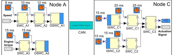
4.3. Analysis of Distributed Transactions with Branches
Saad Mubeen, Jukka M ¨aki-Turja, and Mikael Sj ¨odin
andm2that are received byISWC C1 andISWC C2 in node C respectively. Hence, there are two DTs that have different initiators but a single terminator, i.e.,SWC C3 as shown below.
1.SWC A1 →SWC A2 →OSWC A1 →ISWC C1 →SWC C1 →SWC C3
2.SWC A3 →OSWC A2 →ISWC C2 →SWC C2 →SWC C3
Controller Area Network (CAN)
SWC3 OSWC A1 CAN SEND messages ISWC B1 SWC5 SWC6 CAN RECEIVE Port External Event Ext Data Source Data Sink
Controller Area Network (CAN)
Node A Signals SWC1 OSWC_A CAN SEND Ext messages Signals ISWC_B SWC2 SWC3 CAN RECEIVE Node B Data Port Trigger Port External Event Ext Data Source Data Sink
Fig. 6.Two-node DRE system modeled with RCM
Assume that Data Age delay constraint is specified onSWC C3. Also as-sume that the start of this constraint is specified on the component SWC A1
in node A. Therefore, we need to perform end-to-end delay analysis only on the first DT (in the above list). The calculations for Data Age delay require the response time ofSWC C3. However, the response time of this task depends upon the holistic response times of both DTs. In this case, the HRTA plug-in will calculate the holistic response times of all branches whereas the E2EDA plug-in will consider the maximum value among these holistic response times during calculations for the end-to-end delays.
8 ms 16 ms 4 ms
SWC_A SWC_B SWC_C
Sensor Input Data sink
10 ms SWC_A SWC_B SWC_C
Sensor Input Data sink
(a) (b) (c) (a) (b) SWC_A SWC_C SWC_B
Sensor Input Data sink
SWC_E
SWC_D
8 ms 16 ms 4 ms
(d) Node C ISWC_C1 ISWC_C2 Actuation Signal SWC_C1 SWC_C2 SWC_C3 15 ms
15 ms15 ms
20 ms 25 ms
CAN 12 ms
8 ms 10 ms
Speed SWC_A2 OSWC_A1 SWC_A1 15 ms 15 ms SWC_A3 OSWC_A2 Engine torque Node A
Fig. 7.RCM model of a two-node DRE system with branches in distributed transactions
4.4. Analysis of Mixed Task Chains
Instead, we use the second option that reduces the number of paths in mixed chain by combining all tasks belonging to a trigger sub-chain into a single task activated by independent clock. Hence, the reduced mixed chain resem-bles a data chain. For example,SWC B,SWC C andSWC D are combined to a single task (with combined WCETs, offsets, etc.) which is triggered by inde-pendent clock whose period is exactly the same as that of the clock that triggers
SWC B component. The execution time line of the task chain corresponding to
reduced mixed chain of Fig. 5(d) is shown in Fig. 8(b). The corresponding end-to-end delays are also identified. By implementing the second option , we got rid of the so-called “impossible timed paths”. Mixed chains may also exist in the models of DRE systems where they may contain many combinations of data and trigger chains distributed over several nodes. Path reduction in distributed mixed chains is done in a similar fashion.
τB
τC
τD
5 10 15 20 25 τC
0 30
τA
5 10 15 20 25
0 30
5 10 15 20 25
0 30
LIFO LILO (Data Age) FIFO (Data Reaction)
FILO
(b) τA
5 10 15 20 25
0 30
5 10 15 20 25
0 30
τB
Impossible
Timed Path
5 10 15 20 25
0 30
τC
5 10 15 20 25
0 30
τD
5 10 15 20 25 τE
0 30
(a)
Fig. 8.(a) Impossible timed paths in mixed chains (b) Reduction of a mixed chain
4.5. Analysis of the System Containing “Outside” Messages
One of the requirements by the users of the analysis tools was that the HRTA and E2EDA plug-ins should be able to support the analysis of a system that receives messages from unknown senders (from outside of the modeled appli-cation). One motivation behind this requirement may be the integration of two systems that are build using different methodologies and tools. Second motiva-tion could be the integramotiva-tion of legacy systems with newly developed systems. Another motivation could be the requirement for the end-to-end timing analy-sis early during the development. At early stage, the models of some nodes may not be available. However, the signals and messages which these missing nodes are supposed to send and receive might have been decided. Hence, the network is assumed to contain messages whose sender nodes are not devel-oped yet. Similarly, the available nodes may send messages via network to the nodes that will be available at a later stage.
problem, each such message is assumed to be the initiator of the corresponding DT. The transmission type and period (or inhibit time or both) of this message are extracted from the user input (instead of the sending task as in the case of intra-model messages). However, the forward attribute inheritance is valid, i.e., the receiver task will inherit the difference between the worst- and best-case response times of the message as its release jitter.
4.6. Impact of Component Technology on the Analysis Implementation
The design decisions made in the component technology (i.e., RCM) can have indirect impact on the response times computed by the analysis. For exam-ple, design decisions could have impact on WCETs and blocking times which in turn have impact on the response times. In order to implement, integrate and test HRTA and E2EDA, the implementer needs to understand the design model (component technology), analysis model and run-time translation of the design model. In the design model, the architecture of an application is de-scribed in terms of software components, their interconnections and software architectures. Whereas in the analysis model, the application is defined in terms of tasks, transactions, messages and timing parameters. At run-time, a task may correspond to a single component or a chain of components. The run-time translation of a component may differ among different component technologies.
4.7. Direct Cycles in Distributed Transactions
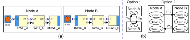
A direct cycle in a DT is formed when any two tasks located on different nodes send messages to each other. When there are direct cycles in a DT, the HRTA may run forever (if deadlines are not specified) because the response times increase in every iteration. Consider a two-node application modeled in RCM as shown in Fig. 9 (a). TheOSWC Acomponent in node A sends a message
m1 to node B where it is received byISWC B. Similarly,OSWC B in node B sends a messagem2 toISWC Ain node A.
There are two options for the run-time allocation of network interface com-ponent (OSWC or ISWC) as shown in Fig. 9 (b). First option is to allocate it to the task that corresponds to the immediate SWC, i.e., the component that receives/sends the signals from/to it. SinceSWC Ais immediately connected to both network interface components in node A, there will be only one task in node A denoted byτAas shown in Fig. 9 (b). Similarly,τB is the run-time
a receiver. No doubt, there is a cycle between the nodes, but not a direct one. Hence, the HRTA may produce converging results, and non-terminating execu-tion of the plug-in may be avoided. It is interesting to note that the requirements and limitations of the analysis implementation may provide feedback to the de-sign decisions concerning the run-time allocation of modeling components.
τB τC τD
5 10 15 20 25
τC
0 30
τA
5 10 15 20 25
0 30
5 10 15 20 25
0 30
LIFO LILO (Data Age) FIFO (Data Reaction)
FILO
(b) τA
5 10 15 20 25
0 30
5 10 15 20 25
0 30
τB
Impossible
Timed Path
5 10 15 20 25
0 30
τC
5 10 15 20 25
0 30
τD
5 10 15 20 25
τE
0 30
(a)
(a)
Node A
ISWC_A SWC_A OSWC_A
Node B
ISWC_B SWC_B OSWC_B
Option 2 (b) m2 Node B τSWC_B τOSWC_B τISWC_B Node A τSWC_A τISWC_A m1 τOSWC_A Node A τA Option 1
m2 m1
Node B
τB
Fig. 9.Options for the run-time allocation of network interface components
4.8. Sequential Execution of Plug-ins in Rubus Plug-in Framework
The in framework in Rubus-ICE allows only sequential execution of plug-ins. There exists a plug-in in Rubus-ICE that can perform RTA of tasks in a node and it is already in the industrial use. There are two options to develop the HRTA plug-in for Rubus-ICE as shown in Fig. 10. The option A supports reusability by building the HRTA in by integrating existing RTA in with two new plug-ins, i.e., one implementing network RTA and the other implementing the HRTA. In this case, the HRTA plug-in will be lightweight. It iteratively uses the analysis results produced by the node and the network RTA plug-ins and accordingly provides new inputs to them until converging holistic response times are ob-tained or the deadlines (if specified) are violated. On the other hand, option B requires the development of the HRTA plug-in from the scratch, i.e, implement-ing the algorithms of node, network and the HRTA. This option does not support any reuse of existing plug-ins.
Node RTA Plug-in
Rubus Builder
Algorithms for RTA of Tasks in a Node Node Timing
Information
Network RTA Plug-in Algorithms for RTA of messages in a Network Network Timing
Information
Rubus-ICE
Rubus Desiner
Modeled DRE Application
ICCM File
End-to-end Timing Model
System Timing Model
Network Timing Model Node Timing
Model HRTA Plug-in
Response Time Analysis of messages in a Network
Holistic Response-Time Analysis
Analysis Results HRTA Plug-in
Algorithms for HRTA
End-to-end Timing Information
Rubus Builder
HRTA Plug-in Algorithms for RTA of Tasks
in a Node
Algorithms for RTA of messages
in a Network
Algorithms for HRTA
End-to-end Timing Information
Analysis Results
Analysis Results Analysis Results Analysis
Results
Option A Option B
Fig. 10.Options to develop the HRTA Plug-in for Rubus-ICE
Since, option A allows the reuse of a pre-tested and heavyweight node RTA plug-in, it is easy to implement and requires less time for implementation, inte-gration and test compared to option B. However, the implementation method in option A is not supported by the plug-in framework of Rubus-ICE because the plug-ins can only be executed sequentially. Hence, we selected option B for the
implementation of the HRTA. Since E2EDA algorithm is non-iterative, there is no need to build the E2EDA plug-in from the scratch. In fact, the HRTA plug-in can be completely reused as a black box. This means that the response times of tasks, messages and task chains computed by the HRTA plug-in can be used as one of the inputs for the E2EDA plug-in as shown in Fig. 4.
4.9. Analysis of DRE Systems with Multiple Networks
In a DRE system, a node may be connected to more than one network. This type of node is called a gateway node. If a transaction is distributed over more than one network, the computation of its holistic response time involves the analysis of more than one network. Such transaction is divided into sub- trans-actions (each having a single network) which are analyzed separately in the first step. In the second step, the attribute inheritance is carried out (see Section 3.3) and the sub-transactions are analyzed again. The second step is repeated until the response times converge or the deadlines (if specified) are violated. Although, we analyze the sub-transactions separately, the multi-step analysis (especially attribute inheritance step) makes the overall analysis to be holis-tic. The implemented HRTA does not support the analysis of a transaction that is distributed cyclically on multiple networks, i.e., the transactions that is dis-tributed over more than one network while its first and last tasks are located on the same network. Since, the E2EDA plug-in receives the response times from the HRTA plug-in, it does not need to split the system into sub-systems.
4.10. Specification of Delay Constraints on Data Paths
One issue that concerns both modeling and analysis is how to specify the de-lay constraints on data paths in both data and mixed chains. This is important because the delay constraints specified in the modeled application have to be extracted in the timing model and the end-to-end delays have to be computed only for the specified data path(s) by the E2EDA plug-in. For this purpose, we in-troduce start and end objects for each of the four delay constraints (discussed in Subsection 3.2) in the component technology. The constraint object has a meaningful name, and start and end points along a data path. Fig. 11 shows the “Data Age” delay constraint specified on a sensor-actuator data path. Sim-ilarly, there are start and end objects for “Data Reaction”, “LIFO” and “FILO” delays. A delay constraint can also be distributed over several nodes. Another useful method for specifying the delay constraints is by selecting each compo-nent (e.g., with mouse click) along the data path.
4.11. Presentation of Analysis Results
times of all tasks, messages and DTs in the system because it may contain a lot of useless information (if the user is not interested in all of it). A way around this problem is to provide the end-to-end response times and delays of only those tasks and DTs which have deadline requirements and delay constraints (specified by the user) or which produce control signals for external actuators. Apart from this, we also provide an option for the user to get detailed analysis results from both the HRTA and E2EDA plug-ins. The analysis report also shows network utilization which is defined as the sum of the ratio of transmission time to the corresponding period (or minimum-update time) for all messages [32].
Fig. 11.Age delay constraint specified on a data path
4.12. Interaction between the User and the HRTA Plug-in
We feel that it is important to display the number of iterations, running time and over all progress of the plug-in during its execution. Further, the user should be able to interact with the plug-in, i.e., stop, rerun or exit the plug-in at any time.
4.13. Suggestions to Improve Schedulability Based on Analysis Results
If the analysis results indicate that the modeled system is unschedulable, it can be interesting if the HRTA plug-in is able to provide suggestions (e.g., by varying system parameters) guiding the user to make the system schedulable. However, it is not trivial to provide such feedback because there can be so many reasons behind the system being not schedulable. Another interesting and related feature would be to provide a trace analyzer as another plug-in that can be used after system has been developed. This analyzer will record the execution of the actual system and then present a graphical comparison of the trace with response times of tasks and messages; holistic response times of trigger, data and mixed chains; and end-to-end delays of data and mixed chains. Based on such comparisons, the user may have better understanding of how the schedulability of the system can be improved. The support for this type of feedback in the HRTA plug-in will be provided in the future.
4.14. Continuous Collaboration between Integrator and Implementer
and the implementer for the verification of the plug-ins. Examples of small DRE systems with varying architectures were created for the verification. The im-plementer had to verify these examples by hand. The integration testing and verification of the HRTA plug-in was non-trivial and most tedious activity.
5.
Automotive Application Case Study
We provide a proof of concept for the analyses that we implemented in the Rubus-ICE by conducting the automotive-application case study. First, we model Autonomous Cruise Control (ACC) system with RCM using Rubus-ICE. Then, we analyze the modeled ACC system using the HRTA and E2EDA plug-ins.
5.1. Autonomous Cruise Control System
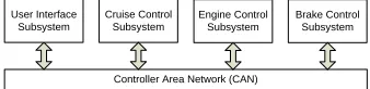
A Cruise Control (CC) system is an automotive feature that allows a vehicle to automatically maintain a steady speed to the value that is preset by the driver. It uses velocity feedback from the speed sensor (e.g., a speedometer) and ac-cordingly controls the engine throttle. However, it does not take into account traffic conditions around the vehicle. Whereas, an Autonomous Cruise Control (ACC) system allows the CC of the vehicle to adapt itself to the traffic environ-ment without communicating (cooperating) with the surrounding vehicles. Often, it uses a radar to create a feedback of distance to and velocity of the preceding vehicle. Based on the feedback, it either reduces the vehicle speed to keep a safe distance and time gap from the preceding vehicle or accelerates the ve-hicle to match the preset speed specified by the driver [41]. The ACC system may be divided into four subsystems, i.e., Cruise Control (CC), Engine Control (EC), Brake Control (BC) and User Interface (UI) [14] as shown in Fig. 12. The subsystems communicate with each other via the CAN network.
Controller Area Network (CAN)
Brake Control Subsystem Engine Control
Subsystem Cruise Control
Subsystem User Interface
Subsystem
Fig. 12.Block diagram of Autonomous Cruise Control System
the CC functionality. It reads input from the proximity sensor (e.g., radar) and processes it to determine the presence of a vehicle in front of it. Moreover, it processes the radar signals along with the information received from other sub-systems such as vehicle speed to determine its distance from the preceding vehicle. Accordingly, it sends control information to the BC and EC subsystems to adjust the speed of the vehicle with the cruising speed or clearing distance from the preceding vehicle. It also receives the status of manual brake sensor from the BC subsystem. If brakes are pressed manually then the CC function-ality is disabled. It also sends status messages to the UI subsystem.
Engine Control (EC) Subsystem. The EC subsystem is responsible for con-trolling the vehicle speed by adjusting engine throttle. It reads sensor input and accordingly determines engine torque. It receives CAN messages from other subsystems that include information regarding vehicle speed, status of manual brake sensor, and input information processed by the UI system. Based on this information, it determines whether to increase or decrease engine throttle. It then sends new throttle position to the actuators that control engine throttle. Brake Control (BC) Subsystem. The BC subsystem receives inputs from sen-sor for manual brakes status and linear and angular speed sensen-sors connected to all wheels. It also receives a CAN message that includes control informa-tion processed by the CC subsystem. Based on this feedback, it computes new vehicle speed. Accordingly, it produces control signals and sends them to the brake actuators and brake light controllers. It also sends CAN messages to other subsystems that carry status of manual brake, vehicle speed and RPM.
5.2. Modeling of ACC System with RCM in Rubus-ICE
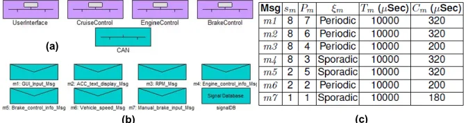
In RCM, we model each subsystem as a separate node connected to a CAN network as shown in Fig. 13(a). The selected speed of the CAN bus is 500 kbps. The extended frame format is selected, i.e., each frame will use 29-bit identifier [24]. The ACC system is modeled with trigger, data and mixed chains.
There are seven CAN messages in the system as shown in Fig. 13(b). A signal data base “signalDB” that contains all the signals sent to the network is also shown. Each signal in the signalDB is linked to one or more messages. The extracted attributes of all messages including data size (sm), priority (Pm),
transmission type (ξm) and period or inhibit time (Tm) are listed in the table
Saad Mubeen, Jukka M ¨aki-Turja, and Mikael Sj ¨odin
m4 andm2 to the CAN network as shown in Fig. 16(b). The Cruise Control as-sembly contains two SWCs: one handles the input and CC mode signals while the other processes the received information and produces control messages for the other nodes. The internal model of this assembly is shown in Fig. 17.
(c) (d)
(a)
(b) (c)
Fig. 13.(a) RCM model of ACC system, (b) RCM model of CAN messages and signal database, (c) message attributes extracted from the model
(a) (b)
(c) (d)
Fig. 14.RCM model of (a) CC node, (b) EC node, (c) BC node, (d) UI node
(a) (b)
(c) (d)
(a)
(b) (c)
(a) (b)
Fig. 15.CC node: Internal model of the Input from Sensors assembly
Internal Model of EC Node in RCM. The EC node is modeled with four assem-blies as shown in Fig. 14(b). The Input from Sensors assembly contains one SWC that reads the sensor values corresponding to the engine torque as shown in Fig. 18(a). The Input from CAN assembly contains three ISWCs, i.e., Vehi-cle Speed Msg ISWC, Engine control info Msg ISWC and Manual brake input Msg ISWC as shown in Fig. 18(b). These components receive messagesm6,
Support for end-to-end response-time and delay analysis in the industrial tool
engine throttle. These components are part of a distributed mixed chain that we will analyze along with other distributed mixed chains in the next subsections.
Sensor Input Data sink
Sensor Input Data sink
(a) (b)
(c)
(a) (b)
SWC_A
SWC_C SWC_B
Sensor Input Data sink
SWC_E
SWC_D
8 ms 16 ms 4 ms
(d)
Node C
ISWC_C1
ISWC_C2
Actuation Signal SWC_C1
SWC_C2
SWC_C3 15 ms
15 ms15 ms
20 ms 25 ms
CAN 12 ms
8 ms 10 ms
Speed
SWC_A2 OSWC_A1 SWC_A1
15 ms 15 ms
SWC_A3 OSWC_A2
Engine torque
Node A
(a) (b)
Fig. 16.CC node: Internal model of assemblies (a) Input from CAN, (b) Output to CAN
Fig. 17.CC node: SWCs comprising the Cruise Control assembly
(a)
(b)
(c)
(c)
(b) (a)
Fig. 18. EC node: Internal model of assemblies (a) Input from Sensors, (b) In-put from CAN, (c) OutIn-put to Actuators
Interface (GUI), but also computes control signals for the other nodes. The In-put from Sensors assembly contains two SWCs as shown in Fig. 22(a). One of them reads the sensor values that correspond to the state of the cruise control switch on the steering wheel. The other SWC reads the sensor values that cor-respond to the vehicle cruising speed set by the driver. The Input from CAN as-sembly contains four ISWC components, i.e., Vehicle Speed Msg ISWC, RPM Msg ISWC, Manual brake input Msg ISWC and ACC text display Msg ISWC as shown in Fig. 22(b). These components receive messagesm6,m3,m7 and
m2from the CAN respectively. The third assembly, i.e., Output to CAN Periodic sends a message m1 to the CAN via the OSWC component as shown in Fig. 22(c). The fourth assembly, i.e., GUI Display Asm contains one SWC, i.e., GUIdisplay component as shown in Fig. 23. This component sends the signals (corresponding to updated information) to GUI in the car.
Fig. 19.EC node: SWCs comprising the Engine Control assembly
(a)
(a)
(a)
(c)
(b) (a)
Fig. 20. BC node: Internal model of assemblies (a) Input from Sensors, (b) In-put from CAN, (c) OutIn-put to CAN
5.3. Modeling of End-to-end Deadline Requirements
We specify end-to-end deadline requirements on four DTs in the ACC system using the deadline object in RCM. All these DTs, i.e., DT1, DT2, DT3and DT4 are distributed mixed chains as shown in Table 1. All these chains have one common initiator, i.e., their first task corresponds to the SWC that reads radar signal which is denoted by RadarSignalInput and located in the CC node as shown in Fig. 15. The last tasks of DT1 and DT2 are located in the BC node. These tasks correspond to the SWCsSetBrakeSignalandSetBrakeLightSignal
Support for end-to-end response-time and delay analysis in the industrial tool
in Fig. 14(b). It produces control signal for the engine throttle actuator. The last task of DT4corresponds toGUIdisplay SWC and is located in the UI node as shown in Fig. 14(d). This task provides display information for the driver.
(b)
(c)
(c)
(b) (a)
(a)
(b)
Fig. 21.BC node: Model of assemblies (a) Brake Control (b) Output to Actuators
(a)
(b) (c)
Fig. 22. UI node: Internal model of assemblies (a) Input from Sensors, (b) In-put from CAN, (c) OutIn-put to CAN Periodic
(a)
(b) (c)
Fig. 23.UI node: Internal model of the GUI Display Asm assembly
1. DT1:RadarSignalInput →InputAndModeControl →InfoProcessing→
Brake control info Msg OSWC →message:m5 →
Brake control info Msg ISWC →BrakeInputInfoProcessing →
BrakeController→SetBrakeSignal SWC
2. DT2:RadarSignalInput →InputAndModeControl →InfoProcessing→
Brake control info Msg OSWC →message:m5 →
Brake control info Msg ISWC →BrakeInputInfoProcessing →
BrakeController→SetBrakeLightSignal SWC
3. DT3:RadarSignalInput →InputAndModeControl →InfoProcessing→
Engine control info Msg OSWC →message:m4 →
Engine control info Msg ISWC →EngineInputInformationProcessing→
ThrottleControl→SetThrottlePosition
4. DT4:RadarSignalInput →InputAndModeControl →InfoProcessing→
ACC text display Msg OSWC →message:m2 →
ACC text display Msg ISWC →GUI Control →GUIdisplay
5.4. Analysis of ACC System using the HRTA and E2EDA Plug-ins
The run-time allocation of all the components in the model of the ACC system results in 19 transactions, 36 tasks and 7 messages. We provide the analysis results of only those transactions on which deadline requirements or delay con-straints are specified. The transmission times (Cm) of all messages computed
by the HRTA plug-in are listed in the table shown in Fig. 13(c). The WCET of each component in the modeled ACC system is selected from the range of 10-60µSec. The HRTA plug-in analyzes all four DTs (discussed in the previous subsection). Once the HRTA plug-in has completed its execution and produced analysis results then the E2EDA plug-in analyzes only those DTs on which end-to-end delay constraints are specified (i.e., all four DTs).
The analysis report in Table 1 provides worst-case holistic response times of the four distributed mixed chains using the HRTA plug-in. The correspond-ing deadlines are also shown. The response time of a DT is counted from the activation of the first task to the completion of the last task in the chain. The response times of these four DTs correspond to the production of control sig-nals for brake actuators, brake lights controllers, engine throttle actuator and GUI. The analysis report produced by the E2EDA plug-in is shown in Table 2. It lists four end-to-end delays calculated for each DT. The corresponding speci-fied delay constraints are also listed in the table. By comparing the end-to-end deadlines and specified delay constraints with the calculated holistic response times and end-to-end delays in Tables 1 and 2 respectively, we see that the modeled ACC system meets all of its deadlines.
6.
Conclusion and Future Work
networks without a need for changing the end-to-end analysis algorithms. With the implementation of these plug-ins, Rubus-ICE is able to support distributed end-to-end timing analysis of trigger flows as well as asynchronous data flows which are common in automotive embedded systems.
Table 1.Analysis report by the HRTA plug-in
Distributed Chain Control Signal Produced Deadline Holistic Response
Transaction Type by the Chain (µSec) Time (µSec)
DT1 Mixed Chain SetBrakeSignal 1000 220
DT2 Mixed Chain SetBrakeLightSignal 1000 280
DT3 Mixed Chain SetThrottlePosition 1000 130
DT4 Mixed Chain GUIdisplay 1500 345
Table 2.Analysis report by the E2EDA plug-in
Distributed Transaction DT1 DT2 DT3 DT4
Specified Age Delay Constraint(µSec) 5000 5000 5000 5000
Calculated Age Delay (µSec) 4220 4280 4130 4345
Specified Reaction Delay Constraint(µSec) 10000 10000 10000 10000
Calculated Reaction Delay (µSec) 8220 8280 8130 8345
Specified LIFO Delay Constraint(µSec) 1000 1000 1000 1500
Calculated LIFO Delay (µSec) 220 280 130 345
Specified FILO Delay Constraint(µSec) 15000 15000 15000 15000
Calculated FILO Delay (µSec) 12220 12280 12130 12345
There are many challenges faced by the implementer when state-of-the-art real-time analyses like HRTA and E2EDA are transferred to the industrial tools. The implementer has to not only code and implement the analyses in the tools, but also deal with various challenging issues in an effective way with respect to time and cost. We discussed and solved several issues that we faced during the implementation, integration and evaluation of the plug-ins. The experience gained by dealing with the implementation challenges provided a feed back to the component technology. We found the integration testing to be a tedious and non-trivial activity. Our experience of implementing, integrating and evaluating these plug-ins shows that a considerable amount of work and time is required to transfer complex real-time analysis results to the industrial tools.
We provided a proof of concept by modeling the ACC system with compo-nent-based approach using the existing industrial component model (Rubus Component Model) and analyzing it with the HRTA and E2EDA plug-ins.
We believe that most of the problems discussed in this paper are generally applicable when real-time analysis is transferred to any industrial or academic tool suite. The contributions in this paper may provide guidance for the imple-mentation of other complex real-time analysis techniques in any industrial tool suite that supports plug-in framework for the integration of new tools and allows component-based development of distributed real-time embedded systems.
with FIFO and work-conserving queues [18, 20], and RTA of CAN with FIFO Queues for Mixed Messages [36] within HRTA plug-in. We also plan to inte-grate the stand alone analyzer, that we developed for the analysis of mixed messages with offsets [38], with the HRTA plug-in.
References
1. Arcticus Systems, http://www.arcticus-systems.com
2. BAE Systems H ¨agglunds, http://www.baesystems.com/hagglunds
3. CANoe. www.vector.com/portal/medien/cmc/info/canoe productinformation en.pdf 4. CANopen Application Layer and Communication Profile. CiA Draft Standard 301.
Version 4.02. February 13, 2002, http://www.can-cia.org/index.php?id=440 5. Knorr-bremse, web page, http://www.knorr-bremse.com
6. MAST–Modeling and Analysis Suite for RT Applications, http://mast.unican.es 7. Mecel, web page, http://www.mecel.se
8. RAPID RMA: The Art of Modeling Real-Time Systems, www.tripac.com/rapid-rma 9. Requirements on Communication, Release 3.0, Revision 7, Ver. 2.2.0. The
AU-TOSAR Consortium, September, 2010, www.autosar.org 10. The Volcano Family, http://www.mentor.com/products/vnd 11. Vector. http://www.vector.com
12. Volcano Network Architect. Mentor Graphics, http://www.mentor.com/products/vnd/ communication-management/vna
13. Volvo Construction Equipment, http://www.volvoce.com
14. Adaptive Cruise Control System Overview. In: Workshop of Software System Safety Working Group (April 2005), Anaheim, California, USA
15. H ¨agglunds Controller Area Network (HCAN), Network Implementation Specification. BAE Systems H ¨agglunds, Sweden (internal document) (April 2009)
16. TIMMO Methodology , Version 2. TIMMO (TIMing MOdel), Deliverable 7 (Oct 2009) 17. Audsley, N., Burns, A., Davis, R., Tindell, K., Wellings, A.: Fixed priority pre-emptive
scheduling:an historic perspective. Real-Time Systems 8(2/3), 173–198 (1995) 18. Davis, R., Navet, N.: Controller Area Network (CAN) Schedulability Analysis for
Mes-sages with Arbitrary Deadlines in FIFO and Work-Conserving Queues. In: 9th IEEE International Workshop on Factory Communication Systems. pp. 33 –42 (May 2012) 19. Davis, R., Burns, A., Bril, R., Lukkien, J.: Controller Area Network (CAN)
schedula-bility analysis: Refuted, revisited and revised. RTS 35, 239–272 (2007)
20. Davis, R.I., Kollmann, S., Pollex, V., Slomka, F.: Controller Area Network (CAN) Schedulability Analysis with FIFO queues. In: ECRTS 2011
21. Feiertag, N., Richter, K., Nordlander, J., Jonsson, J.: A Compositional Framework for End-to-End Path Delay Calculation of Automotive Systems under Different Path Semantics. In: CRTS, 2008
22. Hagner, M., Goltz, U.: Integration of scheduling analysis into uml based develop-ment processes through model transformation. In: International Multi-conference on Computer Science and Information Technology (IMCSIT). pp. 797 –804 (Oct 2010) 23. Hamann, A., Henia, R., Racu, R., Jersak, M., Richter, K., Ernst, R.: Symta/s -
sym-bolic timing analysis for systems (2004)
24. ISO 11898-1: Road Vehicles interchange of digital information controller area net-work (CAN) for high-speed communication, ISO Standard-11898, Nov. 1993. 25. Joseph, M., Pandya, P.: Finding Response Times in a Real-Time System. The
26. K. H ¨anninen et.al.: Framework for real-time analysis in Rubus-ICE. In: 13th IEEE Conference on Emerging Technologies and Factory Automation) (2008)
27. K. H ¨anninen et.al.: The Rubus Component Model for Resource Constrained Real-Time Systems. In: 3rd IEEE Symposium on Industrial Embedded Systems (2008) 28. Liu, C., Layland, J.: Scheduling algorithms for multi-programming in a hard-real-time
environment. ACM 20(1), 46–61 (1973)
29. M ¨aki-Turja, J., , Nolin, M.: Tighter response-times for tasks with offsets. In: Real-time and Embedded Computing Systems and Applications Conference (August 2004) 30. Mubeen, S.: Modeling and timing analysis of industrial component-based distributed
real-time embedded systems. Licentiate thesis, M ¨alardalen University (January 2012), http://www.mrtc.mdh.se/index.php?choice=publications&id=2748
31. Mubeen, S., M ¨aki-Turja, J., Sj ¨odin, M.: Extending response-time analysis of con-troller area network (CAN) with FIFO queues for mixed messages. In: 16th IEEE Conference on Emerging Technologies and Factory Automation (September 2011) 32. Mubeen, S., M ¨aki-Turja, J., Sj ¨odin, M.: Extending schedulability analysis of controller
area network (CAN) for mixed (periodic/sporadic) messages. In: 16th IEEE Confer-ence on Emerging Technologies and Factory Automation (ETFA) (September 2011) 33. Mubeen, S., M ¨aki-Turja, J., Sj ¨odin, M.: Extraction of end-to-end timing model from component-based distributed real-time embedded systems. In: Time Analysis and Model-Based Design, from Functional Models to Distributed Deployments (TiMoBD) workshop located at Embedded Systems Week. pp. 1–6. Springer (October 2011) 34. Mubeen, S., M ¨aki-Turja, J., Sj ¨odin, M.: Implementation of Holistic Response-Time
Analysis in Rubus-ICE: Preliminary Findings, Issues and Experiences. In: The 32nd IEEE Real-Time Systems Symposium, WIP Session. pp. 9–12 (December 2011) 35. Mubeen, S., M ¨aki-Turja, J., Sj ¨odin, M.: Tracing event chains for holistic
response-time analysis of component-based distributed real-response-time systems. SIGBED Review 8, 48–51 (September 2011), http://doi.acm.org/10.1145/2038617.2038628
36. Mubeen, S., M ¨aki-Turja, J., Sj ¨odin, M.: Response-Time Analysis of Mixed Messages in Controller Area Network with Priority- and FIFO-Queued Nodes. In: 9th IEEE International Workshop on Factory Communication Systems (WFCS) (May 2012) 37. Mubeen, S., M ¨aki-Turja, J., Sj ¨odin, M.: Support for Holistic Response-time Analysis
in an Industrial Tool Suite: Implementation Issues, Experiences and a Case Study. In: 19th IEEE Conference on Engineering of Computer Based Systems (ECBS). pp. 210 –221 (April 2012)
38. Mubeen, S., M ¨aki-Turja, J., Sj ¨odin, M.: Worst-case response-time analysis for mixed messages with offsets in controller area network. In: 17th IEEE Conference on Emerging Technologies and Factory Automation (ETFA) (September 2012) 39. Mubeen, S., M ¨aki-Turja, J., Sj ¨odin, M., Carlson, J.: Analyzable modeling of legacy
communication in component-based distributed embedded systems. In: 37th Eu-romicro Conference on Software Engineering and Advanced Applications (SEAA). pp. 229–238 (September 2011)
40. Nolin, M., M ¨aki-Turja, J., H ¨anninen, K.: Achieving Industrial Strength Timing Predic-tions of Embedded System Behavior. In: ESA. pp. 173–178 (2008)
41. P. Berggren: Autonomous Cruise Control for Chalmers Vehicle Simulator. Master’s thesis, Dept. of Signals and Systems, Chalmers University of Technology (2008) 42. Palencia, J., Harbour, M.G.: Schedulability Analysis for Tasks with Static and
Dy-namic Offsets. IEEE International Symposium on Real-Time Systems p. 26 (1998) 43. Rajeev, A.C., Mohalik, S., Dixit, M.G., Chokshi, D.B., Ramesh, S.: Schedulability