Modeling queueing systems

(1)

CSUSB ScholarWorks

Theses Digitization Project John M. Pfau Library

2006

Angela Zoi Leontas

Follow this and additional works at: https://scholarworks.lib.csusb.edu/etd-project

Part of the Mathematics Commons

Recommended Citation Recommended Citation

Leontas, Angela Zoi, "Modeling queueing systems" (2006). Theses Digitization Project. 3101.

https://scholarworks.lib.csusb.edu/etd-project/3101

(2)

A Thesis

Presented to the

Faculty of

California State University,

San Bernardino

In Partial Fulfillment

of the Requirements for the Degree

Master of Arts

hi

Mathematics

by

Angela Zoi Leontas

(3)

A Thesis

Presented to the

Faculty of

California State University,

San Bernardino

by

Angela Zoi Leontas

June 2006

Approved by:

Peter Williams, Chair, Department of Mathematics

Date 1 '

J. T. Hallett

(4)

ABSTRACT

The main objective of this project is to introduce the theory of queueing systems

and to demonstrate its applicability to real life problems. In the first chapter, we discuss the

Markovian property and measures of effectiveness for queueing systems with exponential

interarrival and service times. This information is used to optimize the performance of

the given system. The second chapter of this project is concerned with queueing systems

with exponential interarrival times, Erlang service times, and a single server. The system

performance measures for this queueing system are derived. An appropriate example model

is constructed and investigated. Chapter three discusses different goodness-of-fit tests that

can be used to determine whether the exponential distribution is appropriate for a given set

of data. Advantages and disadvantages of using different goodness-of-fit tests are discussed

and relevant examples are given. Simulation is a method of analyzing queueing systems

which is an alternative to the analytical approach. In the fourth chapter, a single server

queueing system with exponential interarrival times and Erlang service times is simulated

(5)

ACKNOWLEDGEMENTS

I would like to thank the Lord Jesus Christ who is my source of inspiration and

life. He has blessed me by placing many special people in my life to share my journey

with me.

I would like to express my sincere appreciation to my advisor, Dr. Nadejda

Dyakevich, for giving so much of her time, energy, and dedication to the successful com

pletion of this thesis. Her knowledge, insight, and countless readings of earlier drafts

have improved this work greatly. Also, I would like to thank Dr. Rolland Trapp and Dr.

Charles Stanton for their support and guidance in this project and throughout my studies

at California State University, San Bernardino.

I am grateful to my family for all their love and support in reaching my goals.

I offer my deepest appreciation and gratitude to my parents, who sacrificed all their life

in order to provide their children with advantages they never had. Many thanks to my

(6)

Chapter 1

Introduction

1.1

Overview

The study of the characteristics of waiting lines, or queues, has many important

applii::ations. One of the first problems studied in the field of queueing theory was telephone

traffic congestion by A. K. Erlang in 1909. Erlang's research sparked interest among

many other mathematicians who extended his work. Up to the 1950's, telephony was

the principal application of this theory. Today, queueing theory is a useful tool in other

important applications such as air traffic control, machine repair, scheduling problems, and

time-sharing.

Terminology and Kendall-Lee Notation

To describe a queueing system, we must specify the arrival and service processes.

The arrival process of most queueing systems is independent of the number of customers

present and may be described by the probability distribution that governs the time between

successive arrivals, called the interarrival time. We will assume that at most one arrival

may occur at any given instant and that the arrival process does not depend on the number

of customers present in the queueing system.

The service process of many systems is also independent of the number of cus

tomers present, and we may specify the service time distribution which describes a cus

tomer's service time. We will assume that the servers do not work any slower or faster

(8)

In this work, we will use the following standard abbreviations for the probability

distributions to describe interarrival and service times:

M = Times are independent, identically distributed random

|

variables having an exponential distribution. ;

Ek = Times are independent, identically distributed random ;

variables having an Erlang distribution with shape parameter A;.

There is a standard notation created by Kendall (1951) for describing many queueing

systems. This notation is used for models in which all arriving customers wait in a single

queue until one of s parallel servers becomes available. There are six characteristics of; the

notation written in the form 1/2/3/4/5/6. The first characteristic describes the nature of

the arrival process. The second describes the nature of the service times. '

The third characteristic is the number, s, of parallel servers. The fourth

cjiar-acteristic describes the queue discipline. In this work, the order in which customers! are

served is first come, first served (FCF5).

The fifth characteristic is the maximum number of customers allowed in the sys

tem,

including customers in line and customers being served. If there is no maximum', we

denote this by oo. The sixth characteristic is the size of the population from which cus

tomers are drawn. We denote this by oo unless the number of potential customers is of the

same order of magnitude as the number of parallel servers. Often, for 1/2/s/FCFS/oo/oo,

the shorthand notation of 1/2/s is used.

System Perform£ince Parameters

Certain characteristics of a queueing system are of particular interest to optimize

its performance. The most important characteristics are as follows:

TTj =

steady-state probability that j

customers are in the system

L = expected number of customers in the system

Lq =

expected number of customers in queue

(9)

Ws — expected time a customer spends in service

A = average number of customers per unit time (arrival rate)

/I =

average number of service completions per unit time (service rate)

p = A/s^ = traffic intensity.

1.2 Birth-Death Processes

We assume that no more than one arrival may occur at any given instant of tirpe.

Define U as the time of arrival of the ith customer. Let Ti =

ti+i —U

be theith interarriyal

time. We

will assume the Ti's are independent, continuous random variables described by

the random variable A.

The

most appropriate distribution for A

is the exponential distribution since

inter-arrival times are not usually very long. The density function of an exponential distributipn

with parameter A is

a{t) =

where A is the arrival rate, measured in units of arrivals per hour. Also, 1/A is defined

as the mean interarrival time.

We know from [Ros02] that the mean and variance of an exponential random

variable are given by

varA = To • ^ ■■ A ■ ' ■'

In this chapter, we assume that service times are exponential. Let p be the service rake

in units of customers per hour. Then,

l/p

is the mean service time,

Another reason that the exponeritial distribution is often used for interarrivpl

times is because of its Markovian property. This property implies that the probability

distribution of the time until the next arrival does not depend on how long it has been

since the last arrival. Throughout this work, we assume that all interarrival times are

(10)

Lemma 1.1 (Markovian Property). If A has an exponential distribution, then for all

nonnegative values oft and h

P(A

>

t

+

h

I

A~

t)

=

P(A

>

h). The proof of the following theorem can be found in [GH85].

Theorem 1.2. Consider an arrival process {N(t), t ~

0},

where N(t) is the number of

arrivals up tot,

N(0)

= 0,

and satisfies the following assumptions:

(i) P( an arrival occurs between time t and t

+

~t)

=

>..~t

+

o(~t), where >.. is a constant

independent of N(t) and limo(~t)/t

=

0;

(ii) P(more than one arrival between t and t

+

~t)

=

o(~t);

(iii) the number of arrivals in non-overlapping time intervals are statistically independent.

Then, interarrival times are exponential with parameter >.. if the number of arrivals that

occur in an interval of length t follows a Poisson distribution with parameter >..t.

Define the number of people present in a queueing system at time

t

to be the state

of the queueing system at time

t.

The probability of j people present in a queueing system

at time t given i people initially present is denoted by I{j (t). For many queueing systems,

I{j

(t)

will approach a limit 7rj for large t. This limit is independent of the number of people

initially in the system. We call 7rj the steady-state probability of state j, or alternatively the equilibrium probability of state j. We will think of 7rj as the probability that at any given time in the distant future, j customers will be present in the system. The 7rj may

also be interpreted as the fraction of time that j customers are present in the queueing

system for some time in the distant future.

A birth-death process satisfies the following three laws:

(i) A birth occurs between time t and t

+

~t with probability Aj~t

+

o(~t), where Aj is called the birth rate in state j. Hence a birth increases the state of the system from j to j

+

l. A birth is equivalent to an arrival to the system.

(ii)

A death occurs between time t and t

+

~t with probability µj~t

+

o(~t), where µj is

called the death rate in state j. Thus a death decreases the system's state from j to j - l.

A death will" be thought of as a service completion. To ensure a non-negative state, we

require µo

=

0.

(11)

The birth-death model is not appropriate when either the interarrival or service

times are not exponential.

Steady-State Probabilities for Birth-Death Processes

We will outline the steps of the derivation of the steady-state probabilities. See

[Win94] for more details.

We relate ~ j (t

+

D..t)

to Pij (t) for small

D..t

by

~j (t

+

D..t)

~ Pij (t)

+

D..t

(>-j-1Pi,j-l (t)

+

µj+lPi,j+l (t) - ~j (t) µj - ~j (t) Aj)

+

o (b..t). We divide both sides by

D..t,

and take the limit as

D..t

-too. For all i and j

2:

1, we have

~/(t)

=

Aj-1~,j-1 (t)

+

µj+lPi,Hl (t) - ~j (t) µj - Pij (t) Aj,

and for j

=

0,

~,o'(t)

=

µ1Pi,1 (t) - >.o~,o (t).

We will use this infinite system of differential equations to obtain the steady-state proba

bilities defined by

1rj ;= lim Pij

(t).

t-+oo

To find the steady-state, we set Pi/(t)

=

0 and acquire

1rj-1Aj-1

+

1rj+iµj+l

=

1rj (>.j

+

µj) (j

2:

1)

1r1µ1

=

1ro>.o.

From the above equations, it follows that

1ro>.o

1r1

-µ1

1ro (>.o>-1) 1r2

µ1µ2

Let

Then,

(12)

In the next section, we apply the theory of birth-death processes to determine

the steady-state probabilities for the M / M / s queueing system and use them to derive

measures of effectiveness for the system.

1.3 Optimization for the

M / M /

s

System

Analysis of queueing systems may be used to answer one of the most important

questions for the system: How can we minimize costs for a particular queueing model?

Also, what is the optimal number of servers to minimize the sum of service costs and delay

costs? These questions are of much interest to employers and thus to the modeler as well.

We will explore these questions along with the relevant theory of the M / M / s model ( recall

that s is the number of servers). If j customers are present in the system and j ~ s, then all j customers are in service and s-j servers are idle. However, if j

>

s, thens customers

are in service and j - s are waiting in the queue. If a person arrives and a server is idle,

he enters service immediately; otherwise, he joins the queue of customers awaiting service.

To model this system as a birth-death process, we remember that the birth rate in state j

is the arrival rate

>.;

i.e. Aj =

>.

for j

2:

0. If j servers are busy, service completions occur at a rate of jµ. Thus, if j customers are present, min

(j,

s) servers will be busy, and so,

µj = min (j,

s)

µ. Therefore, the M / M /

s

model may be described as a birth-death process with parameters

Aj

>.

for j

2:

0

µj jµ forj=0,1, ... ,s

µj - sµ for j

>

s. (1.2) Define

as the traffic intensity.

).

p= sµ

To ensure the stability of the system, p must be less than one.

That is, the arrival rate must be less than the maximum service rate, which is achieved

when all s servers are busy. Otherwise, the queue will tend to grow indefinitely in time

and the system will "blow up" [WA04].

(13)

For j

=

1, 2, ... , s, we have

'Trj

-

7r0Cj

1roAoA1 • • · Aj-1

=

µ1µ2 · · "µj

1ro.\i si

-j! (µi) si

(sp)i 1ro

=

.,

J·

For j

2:

s, we have

'Trj

=

7r0Cj

1ro.\o.\1 · · · Aj-1

-µ1µ2". • µj

1ro.\i si

-

_{s! (}

si-sµi) si

(sp)i 1ro

=

(1.3)

s! (si-s) ·

Note that the steady-state probabilities must add to 1 since at any given time, the system

is in some state. Thus,

00

L'Trj

=

1, j=0

and so

00

1 - L'Trj j=0

s-1 oo

L'Trj

+

L'Trj j=0 j=s

_

~

(sp)i 1ro

+

~

(sp)~ 1ro

~ j! ~ s! (sJ-s)

J=0 3=s

s-1 ( / 8 00

l

- 7ro

[

Ls~

+

:,LI

j=0 J j=s

s-1 (

)j

s ( l s-1 )

l

= '·

7ro

~~

+

~

-

~

pi

[ ~

JI

s! 1-p ~

(14)

which implies

1 _ 1ro [~(sp)i

+

s

8

( - 1 _ 1-p

8) ] ~ j! s! 1 - p 1 - p J=O

s-1

(sp)j

(sp)8

l

7ro _[

I:-.-,

+ '

(1 - ) .

j=O J. s. p

Therefore,

1

7l"Q

= - - - - -

(1.4)

s~ (sp(j -1E!L_

~ j. +sT(I=py

J=O

From equation (1.3), we see that the steady-state probability that all servers are busy (i.e.

j ~ s) is given by

=

~

(sp)i 1ro

P(j

~

s)

~s!

(si-s)

J=S

s 00

=

s

70I:pi

s. .

J=S

·:7°

(t,1-t1)

8 8

_ S 7ro

(-1- 1

_

~

P )

s! 1-p 1-p

(sp)8

7ro

=

(1.5)

s!(l-p)

Now denote the expected number of customers waiting in the queue as Lq, If j customers

are present and j ::; s, none of the customers need to wait in the queue. However, if j

>

s, there will be j - s customers waiting in the queue. Thus,

00

j=s

~

.

(sp)i

7f'O

f='s

(J -

s)

s!

(si-s)

_xs7r0 ~ .

_xj-s

-

µss!

~

(J - s) si-sµi

J=S

_xs7rO

Loo (.

)

j-s

- - - J-S p .

(15)

Changing indices, we obtain

\8 00

/\ 7l"QL

n Lq - - - np

µss!

n=l

A8

7rop

~

(~pn)

µ8 _s! _dp _L..t n=l

(sp) 8

7rop - s! (1-

p)

2 •

Hence, from (1.5), we acquire

Lq

=

p

(j

~ s) p. _(1.6)

1-p

Little's Formula

For -any queueing system in which a steady-state distribution exists, the following

relations hold [Win94]:

L -\W

Note that L ~ Lq

+

Ls and W = Wq

+

W8 • Substituting (1.6) into Lq = AWq and solving

for Wq:

=

Lq

,\

p

(j

~ s)

sµ(l-p)

p

(j

~ s)

(1.7) sµ- ,\ .

Determining W8 and L8 along with applying Little's Formula, we may obtain L and W as

follows: Since W8

=

1/µ, we get

,\

Ls=-. µ

Thus,

L Lq+,\

µ

_ P(j ~ s)p

+~.

(16)

Then, since L

=

AW,

W

=

p (j

~

s)

+

~-sµ - A µ

Example 1. 1. An employer wishes to determine the number of servers that should work on Tuesdays. He approximates a delay cost of $0. 05 for every minute a customer waits in

line. On the average, three customers arrive per minute and it takes a server two minutes

to complete the service. Each server is paid $12.00 per hour. Interarrival times and

service times were found to be exponential. How many servers should the employer have

working on Tuesdays to minimize the sum of service costs and delay costs?

We have

A - 3 customers per minute, and

µ - 0.5 customers per minute.

Since p

=

A/

sµ

must be less than one,

3

1 0.5s

<

implies

s

>

6 servers.

Thus, the employer must have at least seven servers to ensure the stability of the system.

Then, for s

=

7, 8, ... we will compute:

Total expected cost Expected service cost Expected delay cost

Minute Minute

+

Minute

Note that each server is paid 12/60

=

$0.20 per minute. Hence, Expected_ service cost

=

$0.₂0s.

Mmute

Also,

Expected delay cost Expected customers) Expected delay cost)

( (

Minute Minute Customer

- 3

(0.05Wq)

(17)

Then for s

=

7, p ~ 0.86, from (1.4) we get 7fo ~ 0.0015. Thus, using (1.5), P

(j

~ 7) ~

0.62. From (1.7), Wq ~ 1.24 minutes. Hence, for s

=

7,

Expected delay cost ~ $O.l 9, Minute

and so

Total expected cost ~ $1. _ 59 Minute

Computing the service cost per minute for s

=

8 servers in a similar manner, we obtain

$1.60. Therefore, the total expected cost per minute for eight servers cannot possibly be

lower than that of seven servers since the service cost alone for eight servers is more than

(18)

Chapter 2

The Erlang Distribution

When the interarrival times do not fit an exponential distribution function, they

can often be modeled by an Erlang distribution [Win94]. Let T be a continuous random

variable with Erlang density function

R(Rt)k-1_e-Rt

f(t)

=

(k - 1)! '

where R

>

0 is the rate parameter, k is the shape parameter ( a positive integer), and

t

2:

0. The mean and variance are

E(T)

=

~

and

k

var(T)

=

R_{2 ,}

respectively [Win94]. If k

=

1, then f(t)

=

Re-Rt (for t

2:

0), which is an exponential distribution with parameter R. Thus, the exponential distribution is a special case of the

Erlang distribution. More specifically, it is an Erlang type 1. If the interarrival times do

not seem to fit an exponential distribution, we often consider an Erlang distribution with

rate parameter k>.., shape parameter k, and mean 1/

>..

This can provide greater flexibility by being better able to represent the real world [GH85].

The sum of k independent, identically distributed exponential random variables

with mean l/kµ is an Erlang type k distribution [Win94]. The Erlang distribution can

be used to describe queueing models where the service may be a series of k identical phases

(19)

Note that all phases are independent and identical. Also, only one customer at

a time can be in the service process. That is, a customer enters service in phase k, then phase k - 1, and so on. After phase 1 is completed, the customer leaves the system. A

customer must complete all phases of service before the next one may enter phase k of

service.

2.1 The

M / Ek/1

Model

Recall that M / Ek/1 stands for a queueing system with exponential interarrival

times and Erlang-k service times, where k is the number of phases of service. Even if the

queueing system does not have phases of service, it is convenient to analyze it in this way

since each phase may be considered an exponential random variable which allows us to use

the Markovian property.

Let

Pn,i(t)

be the probability of

n

customers in the queueing system with the

customer in service being in phase i, where i

=

1, 2, ... , k. The first phase of service is phase k, the- second is phase k - 1, and so on; the last phase of service is phase 1. A customer leaving phase 1 leaves the system all together.

We can write the following set of difference equations:

Pn,i(t

+

At)

=

Pn,i(t)(l - >.At - kµAt)

+

Pn,i+1(t)kµAt

+Pn-1,i(t)>.At

(n ~ 2; 1

:Si :S k -

1)

. Pn,k(t

+

At) -

Pn,k(t)(l -

>.At -

kµAt)

+

Pn+1,1(t)kµAt

+Pn-1,k(t)>.At

(n ~ 2)

PI,i(t

+

At) - P1,i(t)(l - >.At -

kµAt)

+P1,i+1(t)kµAt

(n

=

1; 1

:Si :S k -

1)

P1,k(t

+

At) - P1,k(t)(l - >.At -

kµAt)

+

P2,1(t)kµAt

+po(t)>.At

(20)

where the probability that an arrival (service eompletion of phase j)

occurs between time

t and time t

+

At

is equal to AAt

+

o(At)

(fe/uAt 4^ o(At)). Note that At

is a,n incremental

element and o(At) becomes negligible when compared to At as At

0, i.e.

At-^D At ;

Therefore, airo(At) terms were ignored in the above difference equations [GH85].

Let us first consider the case when n > 1. There are several ways for the system

to get to state n,

j

(n customers in system with the customer in service being in phase jf,

n > 1 and j = 1,2,..., fc). The system might have been in state n,j at t and had no net

change during At (that is, no arrivals and no departures of phase y). Or the systern nlay

have found itself in state (n -^ 1)

,y and had an arrival, or in state n,

(j

+

1) and hac[ a

service completiort of phase j + 1- If j = k, another possibility is that the system was

state (n

+

l),

l and had a depairture of phase 1

(and thus exiting the system).

The difference equation for n f= 0 may be interpreted as follows: We consider

how the system may get to state 0

(zero customers in the system) at time t At. The

system might have been in state 0

at t and had no arrivals during At, or the system might

have found itself in state 1 and had a service completion (therefore exiting the system)!

The corresponding differential-difference equations are found by taking pn,i(t)\ to

the left hand side, dividing through by At, and taking the limit as At —>• 0. Using (he

definition of the derivative, we obtain

dpn,i(t)

m

= -(A

+

kp,)pn,i(tl +kppn,i+l{t)

+

Apn-l,i(t)

2;1 <i < jfc -1)

-r{X+ k:jj)pnj,(t) 4- fc/ipn+l,l(t) 4- Apn-l,fc(t)

= --(A4-fcM)pi,i(t)4fcm,i+i(^)

< i < k — 1)

= -{\

+

kp)pi^k{t)

+

kpp2,iit) +

Xpo{t)

dt

(n > 2;1 < i < k-l)

dpn,k

(t)

dt

{n > 2) dpi,i{t)

dt

(1 < i < k — 1)

dpi,kit)

dt dpd{t)

= -Xpoit)

+

kppi,iit).

I

(21)

so the steady-state difference equations are

0 - -(>. + kµ)Pn,i + kµpn,i+l + APn-1,i (n ~ 2; 1::;

i::;

k - 1)

0 -(>. + kµ)Pn,k + kµPn+l,1 + APn-1,k (n ~ 2)

0 -(>.

+

kµ)p1,i

+

kµp1,i+1 (1 ::;

i::;

k - 1) 0 - -(>. + kµ)p1,k + kµp2,1 + >.po

0 - ->.po+ kµp1,1- (2.1)

Let the random variable Tq represent the time spent in the queue, where E[Tq]

=

Wq, We remember that the expected time to complete each of k phases of service is 1/kµ

and thus the total expected time for a full service completion is 1/µ. Thus, the expected time a customer spends waiting in line is equal to the expected time for Nq customers in

line plus the remaining service time of the customer in phase

I.

E[Tq]

=

E[Nq]-1

+

E[I]-k 1

µ µ

1 2 k

-p11 +-p12+ .. · +-Plk kµ ' kµ ' kµ '

k+l k+2 k+k

+--p21 +--p22+ .. ·+--P2k

kµ ' kµ ' kµ '

2k + 1 2k + 2 2k + k

+ kµ P3,1 + ~P3,2 + · · · + kµ P3,k

+ .. ·+Po

k(l-1)+1 k(l-1)+2 k(l-l)+k

kµ Pl,1 + kµ Pl,2 + ' ' . + kµ Pl,k

k(2-1)+1 k(2-1)+2 k(2-l)+k

+ kµ P2,1 + kµ P2,2 + · · · + kµ P2,k

k(3-1)+1 k(3-1)+2 k(3-l)+k

+ kµ P3,1 + kµ P3,2 + · · · + kµ P3,k

+ .. ·+po

00

k [k (n - 1)

+

i]

_(2.2)

- ~tr

kµ Pn,i

+

Po,

where Nq is the random number for the number of customers in the queue and I is the

random number representing the phase of service in which the customer being served is

in.

We wish to derive the expected time a customer waits in the queue Wq using (2.1).

(22)

fourth by zk, and the fifth by z0 gives

-(>.

+

kµ)zk(n-l)+iPn,i

+

kµzk(n-l)+iPn,i+l

+

>.zk(n-l)+iPn-1,i where

(n

>

2; 1 ::; i ::; k - 1)

0

=

-(>.

+

kµ)zknPn,k

+

kµzknPn+l,1

+

>.zknPn-1,k (n

2:

2)

0 -(>.

+

kµ)ip1,i

+

kµip1,i+1 (1 ::;

i::;

k - 1)

0

-

-(>.

+

kµ )zkPl,k

+

kµzkp2,1

+

>.zkpo

0

-

->.z0po

+

kµz0p1,1, (2.3}

0

-Let

G(z)

=

ZPl,1

+

z2p1,2

+,,. +

ZkPl,k

+zk+

1P2,1

+

zk+2P2,2

+ · ·, +

Z2kP2,k

+ · · · +

Po

=

k

- L:L>k(n-l)+iPn,i

+

PO·

n=li=l

Expanding each equation in (2.3) and summing up all terms, we have:

O=i(G(z)-po)-(1+

k~)G(z)+po+ k~zkG(z).

Let r

=

>./kµ. Then,

0

= -

1 (G(z) - Po) - (1

+

r) G(z) +Po+ >.rzkG(z). z

It follows that

G

Po(l -

z)

(z)

=

1-z (1-r)

+

rzk+l' where

>. Po= 1- -.

µ

Thus,

'() -[1-z(l+r)+rzk+l]-(1-z)[-(l+r)+(k+l)rzk]

G z

=

[1-z(l+r)+rzk+l]

2

(23)

From (2.2), we conclude

~G'(l)

kµ

1 (k+l)i

kµ 2

(1 -

i)

(k

+

1)>,

2kµ(µ->.)"

Since the total wait time is a sum of the expected wait time in queue and the expected

wait time in service, we have:

w

=

Wq+Ws

1

w:

_q

+

_µ

(k

+

1) >.

+

2k (µ - >.) 2kµ (µ - >.)

Using this together with Little's Formula, we also obtain

Lq

=

>.Wq

(k+l)>.2

2kµ (µ - >.)

and

L >.W

_ >.( (k+l)>.

1)

2kµ (µ - >.)

+

µ

>. ((k

+

1) >.

+

2k (µ - >.)) .

2kµ (µ - >.)

2.2 An Example for

M/

Ek/1

We wish to determine whether the marketing department should rent a slow or

fast copy machine. The department estimates each employee's time to be worth $15.00

per hour. The slow copier rents for $4.00 per hour, and it takes an employee an average

of 10 minutes with a variance of 19 minutes to complete copying. The faster copier rents

for $8.00 per hour, and it takes an employee an average of 6 minutes with a variance

(24)

machine. The interarrival times were found to be exponential. Which machine should

the department rent to minimize the total expected cost per hour?

Let us first analyze the slow copier. Note that

>.

=

4 employees per hour and

1

- 10 minutes per employee

µ

=

1

6

hours per employee,

so

1

1 .

µ emp oyees per mmute 10

6 employees per hour.

Let us check that the copy times satisfy

var T

<

[E (T)]2 •

Since 19

<

102_,_{an Erlang distribution can be fitted to the copy times [Win94]. Let us} determine k.

1 var T

-

_kµ2

1 19

=

k

Uo)2

k ~ 5.26.

Thus, k

=

5 or k

=

6. For k

=

5, var T

=

20, and for k

=

6, var T

=

16.67. Hence,

we choose k = 5 since the observed variance is closest to that achieved with k = 5.

Therefore, the copying times fit an Erlang distribution with rate parameter kµ

=

½

and shape parameter k

=

5. We have an M / E5/l model. We must also check system stability [Win94], i.e.

>.

p =

- <

1

µ

(25)

thus the queueing system is stable.

Now we carry out the calculations (using hours as the time unit) to determine the

total expected cost per hour for the slow copy machine as follows:

Total Expected Cost Expected Service Cost Expected Delay Cost

- - - = - - - + - - - ,

_Hour _Hour _Hour

where

Expected Delay Cost

=

(Expected Employees) (Expected Delay Cost) .

Hour Hour Employee

Thus,

Total Expected Cost

=

₄

+

_{4 (lSW.).}

Hour q

Note that the expected delay cost per hour is the employee's wage per hour. Calculate

Wq as follows:

(k+l),\

2kµ (µ - ,\)

6 (4)

60 (2) 1

5

hours.

Hence, for the slow machine

Total Expected Cost _{_ 4+}₆₀

Hour ,5

=

$16.00.

Thus, the slow copier has an expected cost of $16.00 per hour.

Similarly, we may analyze the fast copy machine. We have

,\ =

4 employees per hour

1

=

6 minutes per employee

µ

1

=

hours per employee 10

1 1 .

µ

=

6

emp oyees per mmute

(26)

Since var T

<

[E (T)]2, or 9

<

62 , an Erlang distribution may be fitted to the copy times.

We also verify that p

=

A/µ= 4/10

<

1, so the system is stable. To find k: 1

var T

=

kµ2

1 9

k

(¼)2

k

-

4.

Similar to the case for the slow copy machine,

Total Expected Cost Expected Service Cost Expected Delay Cost

Hour Hour

+

Hour

=

8+4(15Wq).

Calculate Wq as follows:

(k

+

1) A Wq =

2kµ(µ-A)

5 (4)

-80 (6)

1

= hours. 24

Thus, for the fast copy machine,

Total Expected Cost 60

Hour 8

+

24

$10.50.

Therefore, the fast copier has an expected cost of $10.50 per hour.

Since the total expected cost per hour is $16.00 for the slow machine versus $10.50

for the fast copier, the marketing department should rent the fast copy machine to minimize

the total cost per hour.

Note that we may also determine the expected number of customers in queue

(Lq)

for the slow and fast copy machines using the steady-state formula that we derived. The

slow copier gives

Lq

=

4/5 employees, and the fast copier gives

Lq

=

1/6 employees. Of

(27)

Chapter

3

Model Selection

Finding the appropriate probability distribution that describes a set of data is

imperative for a model to produce meaningful results. For the queueing systems that we

are interested in, determining whether the actual data are consistent with the assumption of

exponential interarrival times and service times is essential. Goodness of fit tests are often

used ~o test a set of data for fitting a probability distribution. The most common tests are

the chi-square goodness of fit test, Kolmogorov-Smirnov test, and Anderson-Darling test.

In this chapter, we will demonstrate how to use these three tests to choose appropriate

probability distributions for the given data set.

All of these tests compare the data to a theoretical distribution ( with the popu

lation mean m replaced by sample mean m). Given

m,

we wish to conduct a hypothesis test to determine whether ti, t2, ... ,tn represent a random sample from a random variable

with a given density function

f(t).

That is, we want to test the following hypotheses:

H0 : t1, t2, ... , tn is a random sample from a random

variable with a given density function

f(t),

Ha

t1, t2, ...,

tn is not a random sample from a random

variable with a given density function

f(t).

Let us consider queueing models in which we want to fit to an exponential distribution.

Suppose the interarrival times of a queueing system have been observed to be t 1 , t 2 , ... , tn,

(28)

of the arrival rate

>.

from the observed data. A common method is using the maximum

likelihood estimate [KPW04].

Definition 3.1. The likelihood function is

n

L(0)

=

IT

P(Tj

=

tj

I

0)

j=l

and the maximum likelihood estimate of 0 is the value that maximizes the likelihood

function.

This estimate is found by setting the objective function L(0) and then determin

ing the parameter value that optimizes the function. We will show that the maximum

likelihood estimate of the arrival rate

>.

is given by

and the mean of interarrival times

1/

>.

=

0 can be estimated by

n I)i ~ -t i=l

0 = i = - - .

n

By the definition of the likelihood function,

n

L(0) =

IT

P(Tj = tj

I

0)

J=l

n

=

ITf(tj

I

0) j=l

=

f:r0-

1

e-t

j=l

-f:!i

- 0-ne i=l o.

Note that when calculating the likelihood function for a single point, we interpret

(29)

Instead of maximizing L (0), we will maximize l (0)

=

ln L (0). This can be done

since both L (0) and l (0) have their maximum point at the same value. Then,

n

I:ti

l(0) - -nln0 - i=l

0

i=l

3.1

Chi-Square Goodness of Fit Test

The first step in a chi-square goodness of fit test is to break up the set of in

terarrival times into k adjacent intervals

[ao, a1), [a1,

a2), ... ,

[ak-1,

ak), where ak

=

oo. Assuming that

f(t)

governs interarriv1;1,l times, we determine the number of expected in

terarrival times, denoted by ej, that are in interval j. To do this, compute the expected

probability Pi of the data that would fall in the jth interval, where

Pi=

L

p(xi)

aj-I9j$a3

and

p

is the mass function of the fitted distribution. Hence ej

=

npj is the expected number of the data that will fall in the jth interval. Denote the number of observed data

in the jth interval

[aj-1,

aj) by Oj- The chi-square test statistic is

0(o· -

e·)2

x2

=

L..J J J

j=l ej

A small test statistic value demonstrates a good fit. This occurs when the observed

interarrival times are near the expected interarrival times.

Given a value of the desired Type I error (rejecting H0 when it is true) a, the

critical value_ is X%-r-l,l-o:' where r is the number of parameters that must be estimated

for the interarrival time distribution. Note that r

=

1 for the exponential distribution.

(30)

Accuracy of a test is an important factor in modeling. The requirements for

accuracy of the · chi-square test are not concrete, but there are a few guidelines that are

often followed: The intervals should be chosen such that Pl

=

p2

= ... =

Pki this is called the equiprobable approach. This is satisfied for 3 ~ k ~ 30 intervals and ej ~ 5 for all j

[Win94], [LK00]. The lack of rigid rules for interval selection for the chi-square goodness

of fit test is one of its major drawbacks.

However, for the equiprobable approach for interval selection, the chi-square test

is said to be unbiased since it is more likely to reject a false null hypothesis than a true one.

If many ej 's are small and not equal, a highly biased yet valid test is possible. According

to [LK00], the equiprobable approach along with the conditions that ej ~ 5 for all j and

k ~ 3 guarantees a valid and unbiased test.

Example 3.1. The interarrival times (in minutes) observed at a bank are as follows (in

ascending order): 0.1, 0.2, 0.2, 0.3, 0.3, 0.5, 0.6, 0.6, 0. 7, 0.8, 0.9, 1.2, 1.5, 1.6, 1.8,

2.2, 2.3, 3.0, 3.5, 3.8, 3.9, 5.3, 6.1, 9.4, 11.0. Use the chi-square goodness of fit test

with a

=

0.05 to determine if it is reasonable

to

conclude that the observations follow an

exponential distribution.

There are 25 observations with a mean arrival rate

5

j;

=

~

=

0.405 arrivals per minute. 2

I:ti

i=l

Now test whether the data are consistent with an exponential random variable, say A, with

density f(t)

=

O.4O5e-o.4ost. Choose k

=

5 intervals to ensure that the probability that an

observation from A falls into each of the five categories is Pj

=

0.20 for 1 ~ j ~ 5. Thus

ej

=

25(0.20)

=

5 for each interval. Then set the interval boundaries. We must first

calculate the cumulative distribution function, F(t), for

A:

F(t)

=

P(A ~

t)

t

J

0.405e-0.40Sxdx

0

(31)

F(a2)

=

P(A

::S

a2)

=

0.40

F(a3)

=

P(A

::S

a3)

=

0.60

F(a4)

= P(A

::S a4)

= 0.80.

From F(t)

=

1 - e-o.4o5t, we can use natural logarithms to solve for

t

as follows:

F(t)

=

l _ e-o.4o5t

ln e-0.405t

=

_{ln(l - F(t))}

ln(l - F(t))

t

-0.405

ln(l -

F(aj))

£ ll . -0.405 or a J.

It follows that

a1

=

0.55, a2

=

1.26, a3

=

2.27, and

a4

=

3.98.

The number of observations in each interval is

01

=

6, 02

=

6, 03

=

4, 04

=

5, and 05

=

4.

Thus,

(6-5)2 (6-5)2 (4-5)2 (5-5)2 (4-5)2

x2 -

₅

+

₅

+

₅

+

₅

+

₅

=

0.20

+

0.20

+

0.20

+

0

+

0.20 0.80.

The critical value is

xl

_0.95

=

7.81, and since

x

2

=

0.80

::S

7.81, we cannot reject the null hypothesis. Hence, with 95% certainty, the null hypothesis is not rejected and the

exponential dfstribution with

>.

=

0.405 arrivals per minute is a plausible model for the

interarrival times. _□

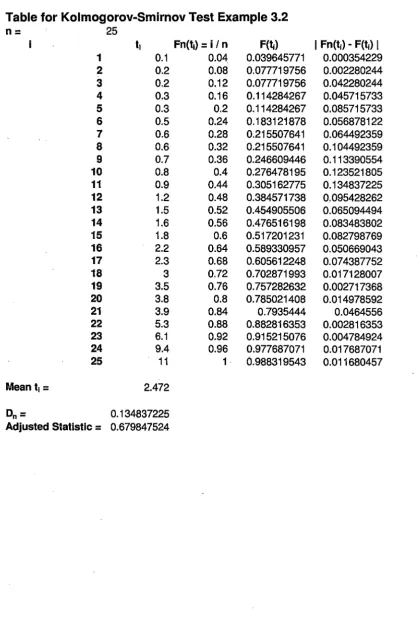
3.2 The Kolmogorov-Smirnov Test

The Kolmogorov-Smirnov (K-S) test is another method that can be used to assess

whether the observations T1, T2, ... , Tn are an independent sample from the exponential

(32)

distribution function. This test has advantages and disadvantages. To perform the test,

the data does not need to be grouped, and hence the problem of interval specification is

eliminated. Although the original K-S test requires all parameters to be known (i.e. the

parameters should not be estimated from the sample data), applying it for discrete or for

any continuous distribution with estimated parameters yields a conservative test. That is,

the actual probability

ci

of rejecting the null hypothesis when it is true is at least as small

as the stated probability a [LK00].

For the K-S statistic, define the empirical distribution function Fn(t) as the right

continuous step function where Fn (T(i))

=

i/n for i

=

1, 2, ... , n. Also, the distribution

function F(t) is assumed to be continuous over the range of data. A natural assessment of

goodness of fit is a measure of closeness of the empirical and fitted distribution functions.

In the case when all parameters are known, the test statistic is the largest vertical distance,

Dn, of Fn(t) and F(t) for all t, where Dn is defined by [KPW04]

Dn

=

sup IFn(t) - F(t)l -t

However, since in our case not all parameters are known (we estimate the mean from the

observations), we will use the adjusted test statistic

0.2) ( c 0.5) ( Dn - -;;;- v n

+

0.26

+

..jn .

Once more, we do not reject H0 if this test statistic is small. A commonly used critical

value for this situation is c1-a

=

1.094 for a= 0.05 [LK00].

Example 3.2. Use the K-8 test with a

=

0.05 on the previous example to determine if it

is reasonable

to

conclude that the observations follow an exponential distribution.

We first set up a table to compute Fn(t), F(t), and IFn(t) - F(t)I for each t. Then

we determine Dn from the table (see Appendix A). Since the critical value is

co.

95

=

1.094

and

0.2) (· /M 0.5 )

D25 -

25

V 25

+

0.26

+

J25

~ 0.6798 :::; 1.094,

(

again we cannot reject the null hypothesis. Hence, using the K-S test with 95% certainty,

the null hypothesis is not rejected and the exponential distribution is a plausible model for

(33)

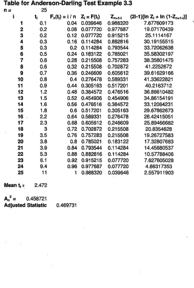
3.3. The Anderson-Darling Test

The Anderson-Darling (A-D) test is a similar test to the K-S test, however it

detects discrepancies in the tails. This is an important characteristic since many distribu

tions mostly differ in their tails [LK00]. Denote the A-D test statistic for the case when

all parameters are known by

00

A;,= n

J

[Fn(t) -

F(t)]

2 'lj;(t)J(t) dt,

-00

where the weight function

1

'lj;(t)

=

F(t)

[1 - F(t)]

Then A~ is the weighted average of the squared differences between the empirical and

model distribution functions. The weights are largest for F(t) close to 0 and 1 (the left

and right tails, respectively). Let Zi = F(T(i)) for i = 1, 2, ... , n. Then the test statistic

for carrying out actual computations can be written as

-{f:(2i-

l)[lnZi

+

ln(l - Zn+1-i)]}

A2 _ n - i=l _ ~

n

The values for Fn(t) and F(t) are calculated the same way as for the K-S test.

Since

A;,

is a weighted distance, we want to reject the null hypothesis if

A;,

is too large. Once again, an adjusted test statistic is available that takes into account that the

mean was estimated from the data. Thus, reject H0 if

( 1

+

0~6)

A;,>

1.326 for a

=

0.05 [LK00].

Example 3.3. Use the A-D test with a

=

0,05· on the previous example to· determine if it

is reasonable to conclude that the observations follow an exponential distribution.

We set up a table to compute Fn(t), Zi, and Zn+l-i for each t (see Appendix B).

Then compute

A;,~

0.4587. Since the critical value is do.95

=

1.326 and

( 0.6)

₁

+

2 _~_0.4697_~_1.326,

25

A25

again we cannot reject the null hypothesis. Thus, using the A-D test with 95% certainty,

the null hypothesis is not rejected and the exponential distribution is a plausible model for

(34)

3.4 Concluding Remarks

We first note that any model is only an approximation of reality, however the

model may still be useful. While selecting a distribution model, it is very important to

follow the principle of parsimony. The principle states that unless there is strong evidence

to use a more complex model, it is preferred to choose a simpler model. Most hypothesis

tests use this principle as well. Unless there is strong evidence to do so, do not reject

the null hypothesis ( and thus claim a more complex model of the population needs to be

found). Finally, it is wise to keep focused on the problem that is to be solved rather than

spend abundant energy searching for the perfect model. The reasoning behind this is that

if a complex model is very close to the observations, there is no guarantee that the model

matches the population from which the data were sampled [KPW04].

There are two main approaches to model selection; they are the judgment-based

and score-based approaches [KPW04]. The judgment-based approach allows for a decision

to be based on the success of particular models in similar situations or on how well the

data compare to the empirical distribution using a graph.

The score-based approach assigns each model a score and the model with the best

score is chosen. Common scores include the lowest value of the Kolmogorov-Smirnov test

statistic, the lowest value of the Anderson-Darling test statistic, the lowest value of the

chi-square goodness of fit test statistic, the highest p-value for the chi-square test, and the

highest value of the likelihood function at its maximum. Overall, the analyst's judgment

is required at the very least in deciding which algorithm to choose.

Each hypothesis test has its advantages and disadvantages. The chi-square good

ness of fit test is commonly used since it may be applied to any hypothesized distribution.

Also, the critical value of the test is easily adjusted depending on the number of param

eters estimated from the data. A valid chi-square test using the equiprobable approach

for interval selection always produces an unbiased test. A test is said to be unbiased if it

is more likely to reject a false null hypothesis than when it is true. However, the major

drawback of this test is the lack of rigid rules for interval selection. In some cases, different

choices of intervals can lead to different conclusions [LK00].

For the Kolmogorov-Smirnov test, the data does not need to be grouped, which

(35)

test statistic when parameters are estimated from the data. The critical values are not

readily available for discrete data and must be computed from difficult formulas. Lastly,

the K-S test statistic gives the same weight to the difference

IFn(t) - F(t)

I

for all values of

t,

but many distributions differ primarily in their tails [LK00].

The Anderson-Darling test has an advantage since its test statistic is a weighted

average where the weights are largest in the tails, unlike the K-S test statistic. Similar

to the K-S test, the A-D test statistic must be adjusted for the case when parameters are

estimated from the data. The critical values for this test also must be computed from

(36)

Chapter 4

Simulation

Simulation is a common method of analyzing queueing systems as an alternative

method to the analytical approach. Perhaps the biggest advantage of simulation is its flex

ibility in the sense that it is possible to create a program for an individual queueing system

without needing as many simplifying assumptions as the analytical method. Queueing

systems with non-exponential service times, a limited capacity waiting room, and many

other situations which are extremely difficult to analyze directly can be explored using

simulation. Simulation should be used when an analytical solution may not be found or

it does not have acceptable approximations [GH85].

Another advantage of simulation is that the user sees the action through time.

Creating simulation models to see the effects of changing system parameters is much more

cost efficient than to change the system in real life. There are three basic phases of

simulation: data generation, bookkeeping, and output analysis. In queueing systems,

the first phase generates the interarrival and service times with appropriately selected

probability distributions. The biggest problem in queueing simulation is bookkeeping.

Bookkeeping involves keeping track of arrivals, departures, busy and idle servers, queue

length, clock time, and status of the server. In other words, timing and bookkeeping is a

challenge [WA04]. The outputs are then analyzed to determine which parameters of the

queueing system should be changed to optimize system performance.

The model that we will consider is a single server queueing system. Customers

arrive at random times to the system. If a customer arrives and the server is busy, the

(37)

simulate the system for a user-defined length of time, called the close time. At this time,

no new arrivals are allowed to enter the system, but customers already present are served.

The simulation terminates when the last customer leaves. This model assumes that the

times between arrivals are exponentially distributed and the service times are Erlang type

k. The purpose of the simulation is to coHect statistics on the system behavior in order to optimize its performance.

4.1 Description of the Simulation

Visual Basic for Applications (VBA) was used to simulate the queueing system

discussed in this chapter. The VBA code takes care of all the timing and statistical

bookkeeping as the simulation runs [Alb00]. The program code may be found in Appendix

C. The key idea of the simulation is one of scheduling events. At any given time, there is

a list of scheduled events of two types. The first type is an arrival. Each time a customer

arrives to the system, the next arrival is scheduled at some random time in the future. The

second type of event is a service completion ( or departure). Each time a customer goes

into service (possibly after waiting in the queue), a departure is scheduled for a random

time in the future.

Generating Exponential and Erlang Type k Service Times

We first want to generate arrival times from the exponential distribution with

parameter .X. We recall that the probability distribution is given by

F(x)

=

1 - e->.t

(t

~ 0).

We use VBA's random number generator to produce a uniform-(0,1) random number r.

Solving the equation

r

=

l - e->.t

for

t

is referred to as the analytical inversion process of generating random variables from

(38)

Note that it does not matter whether we use 1-r or r since both are uniform-(0,1) random

numbers. Thus, we may write

and by taking natural logarithms of both sides, we obtain

lnr

t

=

-T·

This is the formula used in our VBA program to generate random exponential interarrival

times.

To generate Erlang random variables, we may use the fact that an Erlang type k

random variable, x, is the sum of k independent, identically distributed exponential random

variables with mean l/kµ [Win94]. Thus, using VBA's random number generator to

produce uniform-(0,1) random numbers r1, r2, ... ,rk, we have

x

=

t

(-l~ri)

i=l µ

k ln

II

ri

i=l

kµ ,

which is the formula used to generate random Erlang type k service times.

We will now explain the major steps of the program after the user enters the

following inputs: the customer arrival rate, the mean service time per customer, the number

of phases of service, and the closing time.

Step 1:

The program begins by initializing the system. Set the clock time to zero, set the status

of the server to idle, and schedule the first arrival. Go to step 2.

Step 2:

Determine whether the next event will be an arrival or a departure as follows. Find the

minimum of the scheduled event times. If the next event time is that of an arrival, reset

the current clock time to the time of the arrival and go to step 3. If it is a departure,

reset the current clock time to the time of the departure and go to step 4. In either case,

increase the wait times of everyone in the queue by the elapsed time between the previous

(39)

Step 3:

Check to see if the server is busy. If yes, put this arrival at the end of the queue, keeping

track of the arrival time (for later statistics). If the server is idle, place this customer into

service and schedule his departure. Schedule the time of the next arrival. If this time is

after the closing time, do not allow the next arrival and do not schedule any future arrivals.

Go to step 5.

Step 4:

Ifthere is at least one customer in the queue, send the customer from the front of the queue

to the server and record his wait time for later statistics. Move all other customers up one

space in the queue and schedule a departure. If there is no queue, set the server's status to

idle; do not schedule a departure event. Increase the number of served customers by one.

Go to step 5.

Step 5:

If the clock time is greater than the close time and the server is idle, calculate the outputs

and terminate tl:ie program. Otherwise, go to step 2.

The flow chart may be found in Appendix C.

4.2 The M/Ek/1 Example Revisited

Rec.all that in Chapter 2 we considered an example where we used analytical

methods to determine summary measures for the M/Ek/1 model. Here, we want to

compare the theoretical values of the expected wait time in queue (Wq) and the expected

number of customers in queue

(Lq)

found in Example 2.2 with the corresponding values

using a simulation model.

From Example 2.2, we have for the slow copy machine

>. -

4 employees per hour, 1

µ

=

1

6

hours per employee, and

(40)

Theoretical values for the expected wait time and the expected number in queue were

1

Wq

5

hours Lq - 4

5

employees.

For the fast machine we have

1

µ

=

1

-

hours per employee

10

k

=

4 phases of service

Wq 1 hours 24

Lq 1

6

employees.

We use the VBA program to simulate the use of each copy machine.

Inputs and Outputs

There are four inputs for each copier: the employee arrival rate ,\ the mean service

time per employee 1 /µ, the number of phases of service k, and the closing time. At the end of the simulation, we want to display the summary measures, which include: average

time and maximum time in queue, average number and maximum number of employees in

the queue, and the fraction of time that the server is busy. Also, the simulation program

outputs the number of employees processed and the probability distribution of number in

queue.

From [Ros02], we determined to perform one hundred runs for the slow and fast

machines. Each run simulates an eight hour period. Also, by [Win94], we expect the

average of the simulation values to be close to the steady-state values found in Chapter 2.

Slow Copy Machine

We calculated the average wait time and the number in queue to be 0.20055 hours

and 0.80102 employees, respectively. Both averages are very close to the steady-state values

(41)

Fast Copy Machine

We calculated the average wait time and the number in queue to be 0.04158

hours and 0.16644 employees, respectively. Again, both averages are very close to the

steady-state values of 0.041667 hours and 0.166667 employees, respectively.

In summary, simulation allows the user to obtain a realistic analysis of the queue

ing system. This method is commonly used when a queueing model is extremely difficult

or impossible to analyze analytically due to the complexity of the queueing system. Simu

lations allows us to create hypothetical situations without costly real-time experimentation

nor possible loss of clientele due to long lines and long wait times.

(42)

Appendix A

Kolmogorov-Smirnov Test

(43)

Table for Kolmogorov-Smirnov Test Example 3.2

n= 25

ti Fn(t₁₎= i / n F(t1)

I

Fn(t1) - F(t1)

I

1 0.1 0.04, 0.039645771 0.000354229

2 0.2 0.08 0.077719756 0.002280244

3 0.2 0.12 0.077719756 0.042280244

4 0.3 0.16 0.114284267 0.045715733

5 0.3 0.2 0.114284267 0.085715733

6 0.5 0.24 0.183121878 0.056878122

7 0.6 0.28 0.215507641 0.064492359

8 0.6 0.32 0.215507641 0.104492359

9 0.7 0.36 0.246609446 0.113390554

10 0.8 0.4 0.276478195 0.123521805

11 0.9 0.44 0.305162775 0.134837225

12 1.2 0.48 0.384571738 0.095428262

13 1.5 0.52 0.454905506 0.065094494

14 1.6 0.56 0.476516198 0.083483802

15 1.8 0.6 0.517201231 0.082798769

16 2.2 0.64 0.589330957 0.050669043

17 2.3 0.68 0.605612248 0.074387752

18 3 0.72 0. 702871993 0.017128007

19 3.5 0.76 0.757282632 0.002717368

20 3.8 0.8 0.785021408 0.014978592

21 3.9 0.84 0.7935444 0.0464556

22 5.3 0.88 0.882816353 0.002816353

23 6.1 0.92 0.915215076 0.004784924

24 9.4 0.96 0.977687071 0.017687071

25 11 1 0.988319543 0.011680457

Mean t1

=

2.472

Dn= 0.134837225

(44)

Appendix B

(45)

Table for Anderson-Darling Test Example 3.3

n= 25

t1 Fn(t1) = i / n Z1 = F(t1) Zn+1·1 (2i-1 )[In Z1+ In (1 ·Zn+1-1)] 1 0.1 0.04 0.039646 0.988320 7.677609173

'

2 0.2 0.08 0.077720 0.977687 19.07170439

3 0.2 0.12 0.077720 0.915215 25.1114167 4 0.3 0.16 0.114284 0.882816 30.19155515 5 0.3 0.2 0.114284 0.793544 33. 72062638

6 0.5 0.24 0.183122 0.785021 35.58302197

7 0.6 0.28 0.215508 0.757283 38.35801475

8 0.6 0.32 0.215508 0.702872 41.2252672 9 0.7 0.36 0.246609 0.605612 39.61629166 10· 0.8 0.4 0.276478 0.589331 41.33622821 11 0.9 0.44 0.305163 0.517201 40.2163712 12 1.2 0.48 0.384572 0.476516 36.86610482 13 1.5 0.52 0.454906 0.454906 34.86154191 14 1.6 0.56 0.476516 0.384572 33.12064231 15 1.8 0.6 0.517201 0.305163 29.67862673 16 2.2 0.64 0.589331 0.276478 26.42415051 17 2.3 0.68 0.605612 0.246609 25.89466682 18 3 0.72 0:102812 0.215508 20.8354628 19 3.5 0.76 0.757283 0.215508 19.26727583 20 3.8 0.8 0.785021 0.183122 17.32807683 21 3.9 0.84 0.793544 0.114284 14.45680537 22 5.3 0.88 0.882816 0.114284 10.57788406 23 6.1 0.92 0.915215 0.077720 7.627605028 24 9.4 0.96 0.977687 0.077720 4.86317353 25 11 1 0.988320 0.039646 2.557911903

Mean t1=. 2.472

An2=

0.458721

(46)

Appendix C

(47)

YES, process NO, process an arrival a departure

Generate new random numbers

lnlUallze counters and status Indicators

Set clock time = Set clock time= time time of next arrival of next departure

YES

Is the server busy?

Increase the number In queue by 1

NO

Generate Erlang service time (Sn

Generate exponential lnterarrtval time (IT)

YES

Set server status to Idle

Continue

NO

Decrease the number In queue by 1

Generate Erlang service time (Sn

et time of next departure = clock time+ ST

Set time of next arrival = clock time+ IT

Continue

(48)

Code for the Simulation Program

Option Explicit

' Declare system parameters.

' · MeanlATime - mean interarrival time (reciprocal of arrival rate) ' MeanServeTime - mean service time

' MaxAllowedlnQ - maximum number of customers allowed in the queue ' CloseTime - clock time when no future arrivals are accepted

' K -used to generate Erlang number with shape parameter K ' MeanServeTimeDivByK - MeanServeTime/K

' ProdKRand - product of K random numbers between 0 and 1

Dim MeanlA Time As Single, MeanServeTime As Single, _

CloseTime As Single, K As Integer, MeanServeTimeDivByK As Single, ProdKRand As Single

' Declare system status indicators.

NumlnQ - number of customers currently in the queue ServerBusy - the status of the server, 0 for idle, 1 for busy ClockTime - current clock time, where the inital clock time is 0 TimeOtLastEvent - clock time of previous event

EventScheduled(i) - True or False, depending on whether an event of type i is scheduled or not, for i=0,l, where i=0 corresponds to arrivals and i=l corresponds to service completions TimeOfNextEvent(i) - the scheduled clock time of the next event of type i ( only defined when

EventScheduled(i) is True)

Dim NumlnQ As Integer, ServerBusy As Integer, ClockTime A

Modeling queueing systems

CSUSB ScholarWorks

ABSTRACT

ACKNOWLEDGEMENTS

Table of Contents

Acknowledgements iv

Chapter 1

Terminology and Kendall-Lee Notation

In this work, we will use the following standard abbreviations for the probability

systems. This notation is used for models in which all arriving customers wait in a single

including customers in line and customers being served. If there is no maximum', we

steady-state probability that j

Define U as the time of arrival of the ith customer. Let Ti =

where A is the arrival rate, measured in units of arrivals per hour. Also, 1/A is defined

is the mean service time,

Lemma 1.1 (Markovian Property). If A has an exponential distribution, then for all

Steady-State Probabilities for Birth-Death Processes

1.3 Optimization for the

Little's Formula

Chapter 2

Model

where the probability that an arrival (service eompletion of phase j)

(n customers in system with the customer in service being in phase jf,

state (n

have found itself in state 1 and had a service completion (therefore exiting the system)!

dpi,kit)

2.2 An Example for

Chapter

Chi-Square Goodness of Fit Test

3.2 The Kolmogorov-Smirnov Test

3.3. The Anderson-Darling Test

3.4 Concluding Remarks

IFn(t) - F(t)

Chapter 4

4.1 Description of the Simulation

Generating Exponential and Erlang Type k Service Times

4.2 The M/Ek/1 Example Revisited

Inputs and Outputs

Slow Copy Machine

Appendix A

Table for Kolmogorov-Smirnov Test Example 3.2

Appendix B