University of Pennsylvania University of Pennsylvania
ScholarlyCommons
ScholarlyCommons
Publicly Accessible Penn Dissertations
2019
Allosteric Functionality In Mechanical And Flow Networks
Allosteric Functionality In Mechanical And Flow Networks
Jason William Rocks
University of Pennsylvania, [email protected]
Follow this and additional works at: https://repository.upenn.edu/edissertations
Part of the Physics Commons
Recommended Citation Recommended Citation
Rocks, Jason William, "Allosteric Functionality In Mechanical And Flow Networks" (2019). Publicly Accessible Penn Dissertations. 3471.
https://repository.upenn.edu/edissertations/3471
This paper is posted at ScholarlyCommons. https://repository.upenn.edu/edissertations/3471
Allosteric Functionality In Mechanical And Flow Networks
Allosteric Functionality In Mechanical And Flow Networks
AbstractAbstract
Functionally optimized networks abound in nature, efficiently and precisely controlling the propagation of inputs to perform specific tasks. The regulation of protein activity via allostery presents one of the most well-studied examples: such proteins utilize specific conformational or dynamical changes upon the binding of ligands to facilitate communication between distant active sites. Venation networks in animals, plants, fungi and slime molds also display a type of allosteric communication, having the ability to
precisely distribute oxygen and nutrients from a limited number of inputs to locally support growth and activity. Whether via genetic evolution or dynamic adaptation, many of these networks are able to create and control allosteric functionality by locally tuning interactions between nodes. Taking inspiration from this ability to regulate function, we approach allostery as a problem in metamaterials design, asking whether it is possible to create synthetic mechanical and flow networks with allosteric properties. We show that not only is this possible, but is remarkably easy, only requiring a small percentage of
interactions in a network to be tuned. Leveraging the large statistical ensembles of allosteric networks generated in this way, we show that the limits of multifinctionality in both flow and mechanical networks are governed by the same constraint satisfaction phase transition, unifying both systems into a single theoretical framework. Finally, we investigate the underlying mechanisms by which allosteric function is created in flow networks. We show that the relationship between structure and function in flow networks is topological in nature, not depending on local details of the network architecture. The approaches presented in this work for studying allostery in both flow and mechanical networks set the blueprint for understanding and controlling general functional complex networks.
Degree Type Degree Type
Dissertation
Degree Name Degree Name
Doctor of Philosophy (PhD)
Graduate Group Graduate Group
Physics & Astronomy
First Advisor First Advisor
Andrea J. Liu
Keywords Keywords
allostery, flow netoworks, mechanical networks, metamaterials, network optimization, persistent homology
Subject Categories Subject Categories
ALLOSTERIC FUNCTIONALITY IN MECHANICAL AND FLOW
NETWORKS
Jason W. Rocks
A DISSERTATION
in
Physics and Astronomy
Presented to the Faculties of the University of Pennsylvania
in
Partial Fulfillment of the Requirements for the
Degree of Doctor of Philosophy
2019
Andrea J. Liu, Ph.D., Professor of Physics and Astronomy Supervisor of Dissertation
Joshua R. Klein, Ph.D., Professor of Physics and Astronomy Graduate Group Chairperson
Dissertation Committee:
Douglas J. Durian, Ph.D., Professor of Physics and Astronomy Randall D. Kamien, Ph.D., Professor of Physics and Astronomy Eleni Katifori, Ph.D., Assistant Professor of Physics and Astronomy
Dedication
Acknowledgments
I will remember my time in graduate school fondly due to the large number of
won-derful people who have provided me with guidance and support over the years. First
and foremost, I would like to thank my advisor, Andrea Liu. She has been an
in-credibly supportive mentor, both through the good times and the bad, helping to
shape me into both the scientist and the person I am today. Among the many things
she has taught me, one piece of advice in particular will stick with me no matter
what my futures holds: the most important key to success in science is to work on
what you enjoy. I am profoundly grateful that she has been able to overcome the
harsh obstacles she faced in the last few years, and I hope she will continue to be a
cornerstone of my academic life.
I want to thank Eleni Katifori for essentially playing the role of my unofficial advisor
when Andrea was unavailable. At a time when my research felt grueling and stale,
she helped to push me in new scientific directions, reinvigorating my excitement and
enthusiasm for science. Since then she has been a wealth of advice and support. I
at Penn feel like a family. I always appreciated his sense of humor as a self-proclaimed
“social misanthrope” and his ability to create such a light-hearted atmosphere. He
provided me with a lot of guidance and support, teaching me how to cut through
the BS in life. In addition, I want to thank the the other members of my thesis
committee, Doug Durian and Ravi Radhakrishnan, for graciously giving me their
time and advice.
I am extremely lucky to have been a part of the soft matter community at Penn.
It is a truly special place both academically and socially. I want to thank everyone
with whom I had the pleasure of knowing and working with here. In particular, I
would like to thank Kevin Chiou and Carl Goodrich, both of whom were exceptionally
generous and patient with me when I first started graduate school. I learned a lot
of from both of them and really appreciated that they took me under their wings,
providing guidance on some of my first research projects. I also want to thank Henrik
Ronellenfitsch and Sean Ridout for being a pleasure to collaborate with. There are
many, many, many more people that I would like to thank, but I would like to keep
this relatively short, so I will once again thank everyone that has passed through this
community in the last six years for providing me with a place to thrive.
Thanks to Sid Nagel for also helping me learn how to navigate the first research project
in which I had a lead role. I have always appreciated his input and advice as both a
I want to thank my family and friends for always being there for me. Bill Balunas and
Johanna-Laina Fischer, you will always be two of my closest friends. You provided
me with some of my happiest memories and I hope that we remain close friends into
the far future. Thank you to my siblings, Rachel and Brian Rocks - I’m proud of
you both and will always be supportive of you, just as you have been supportive of
me. I want to thank my grandmother, Jean Greenblatt. She taught me to always see
humor in life and I will miss her deeply. Mom and Dad – to be honest, I get a little
teary-eyed writing this – thank you for everything. You two are the main reason I
am the person who I am today. You have always done everything possible to support
me at every step of my life. I am proud to be your son and love both of you from
the bottom of my heart. Finally, I want to thank my partner, Katie Siewert. Thank
you for always being a source of reason and inspiration in my life, helping me to be
the best person I can be. I am lucky to have had someone so special to share this
ABSTRACT
ALLOSTERIC FUNCTIONALITY IN MECHANICAL AND FLOW NETWORKS
Jason W. Rocks
Andrea J. Liu, Ph.D.
Functionally optimized networks abound in nature, efficiently and precisely
control-ling the propagation of inputs to perform specific tasks. The regulation of protein
activity via allostery presents one of the most well-studied examples: such proteins
utilize specific conformational or dynamical changes upon the binding of ligands to
facilitate communication between distant active sites. Venation networks in animals,
plants, fungi and slime molds also display a type of allosteric communication,
hav-ing the ability to precisely distribute oxygen and nutrients from a limited number
of inputs to locally support growth and activity. Whether via genetic evolution or
dynamic adaptation, many of these networks are able to create and control allosteric
functionality by locally tuning interactions between nodes. Taking inspiration from
this ability to regulate function, we approach allostery as a problem in
metamate-rials design, asking whether it is possible to create synthetic mechanical and flow
networks with allosteric properties. We show that not only is this possible, but is
this way, we show that the limits of multifinctionality in both flow and mechanical
networks are governed by the same constraint satisfaction phase transition, unifying
both systems into a single theoretical framework. Finally, we investigate the
under-lying mechanisms by which allosteric function is created in flow networks. We show
that the relationship between structure and function in flow networks is topological
in nature, not depending on local details of the network architecture. The approaches
presented in this work for studying allostery in both flow and mechanical networks set
Contents
1 Introduction 1
2 Designing allotery-inspired response in mechanical networks 8
2.1 Introduction . . . 8
2.2 Theoretical Approach . . . 10
2.3 Computational Results . . . 11
2.4 Experimental Results . . . 17
2.5 Discussion . . . 21
2.6 Materials and Methods . . . 24
2.6.1 Computed Networks and Choice of Source and Target Nodes . 24 2.6.2 Further Details of Theoretical Approach . . . 25
2.6.3 Experimental Networks . . . 30
2.7 Appendix . . . 31
2.7.1 Ghost bonds . . . 31
2.7.2 Creating identical bond stiffnesses . . . 32
2.7.3 Discrete Green’s function . . . 33
2.7.6 Avoiding the introduction of zero modes . . . 39
2.7.7 Removing bonds from SSS and SCS sub-bases . . . 39
2.7.8 Animations . . . 40
2.7.9 Response of experimental networks . . . 41
3 Limits of multifunctionality in tunable networks 46 3.1 Introduction . . . 46
3.2 Network Tuning Protocol . . . 48
3.3 Results . . . 51
3.4 Discussion . . . 53
3.5 Methods . . . 60
3.5.1 Linear Response . . . 60
3.5.2 Bordered Laplacian Formulation . . . 63
3.5.3 Tuning Loss Function . . . 65
3.5.4 Optimization Method . . . 66
3.6 Appendix . . . 68
3.6.1 Variations of the network tuning problem . . . 68
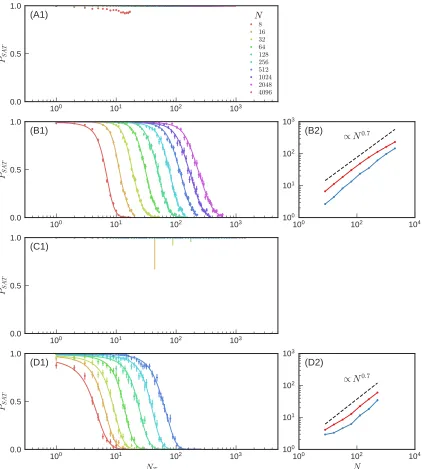
3.6.2 Transition power law fitting and deviations . . . 82
3.6.3 Satisfaction probability error bars . . . 82
3.6.4 Satisfaction probability curve fitting . . . 84
3.6.5 Transition measurements . . . 88
4 The topological basis of function in flow networks 90 4.1 Introduction . . . 90
4.2 Design of Functional Flow Networks . . . 92
4.3 Maximum Tuning Limit (∆ = 1) . . . 95
4.5 Topological Characterization . . . 104
4.6 Structure-Function Relationship . . . 111
4.7 Discussion . . . 118
4.7.1 Summary . . . 118
4.7.2 Experimental Implications and Application . . . 121
4.7.3 Broader Impacts . . . 123
4.8 Appendix . . . 129
4.8.1 Network Tuning Protocol . . . 129
4.8.2 Persistence Algorithm Details . . . 130
5 Conclusions and Future Directions 135 A Mechanical signaling coordinates the embryonic heartbeat 144 A.1 Introduction . . . 144
A.2 Physical model of cardiac mechanical signaling . . . 147
A.3 Results . . . 152
A.3.1 Mechanical signaling model yields contractile wavefronts . . . 152
A.3.2 Mechanical signaling model fits experimental wavefront veloci-ties with physiologically relevant parameters . . . 154
A.3.3 Calculated wavefront strain agrees with experimental observa-tions with no additional fitting parameters . . . 155
A.3.4 Saturating eigenstrain (SE) model is consistent with cell-on-gel measurements with no additional fitting parameters . . . 155
A.3.5 Mechanical signaling model correctly predicts appearance of first heartbeats . . . 156
A.3.6 Conduction interference experiments are consistent with mechanically-coordinated heartbeats . . . 158
A.4.2 Mechanical signaling is consistent with known
mechanosensi-tivity of cardiac myocytes . . . 161
A.4.3 Mechanical vs. electrical signaling in the developing heart . . . 161
A.5 Materials and Methods . . . 163
A.6 Supporting Information . . . 165
A.6.1 Linearized biphasic model . . . 165
A.6.2 Induced strain of Eshelby inclusions . . . 167
A.6.3 Activation condition . . . 173
A.6.4 Tissue strain calculation . . . 176
A.6.5 BGA obstructs intercellular transport in embryonic cardiac tissue178 A.6.6 Small-molecule drugs perfuse embryonic hearts . . . 178
List of Tables
3.1 Variations of tuning problem and corresponding transition exponents 72
A.1 Heart signaling model parameters, references, and values . . . 152
List of Figures
2.1 Allosteric mechanical networks . . . 11
2.2 Allosteric mechanical network tuning statistics . . . 13
2.3 Mechanical network surface strain ratios . . . 15
2.4 Mechanical networks with different types of tuned responses . . . 16
2.5 Additional examples of tuned mechanical networks . . . 17
2.6 Experimental allosteric mechanical networks . . . 18
2.7 Effects of strut widths in experimental mechanical networks . . . 20
2.8 Animation of positive nonlinear response of allosteric mechanical network 42 2.9 Animation of negative nonlinear response of allosteric mechanical net-work . . . 43
2.10 Animation of nonlinear response of periodic allosteric mechanical network 44 2.11 Video of experimental allosteric mechanical network . . . 45
2.12 Nonlinear response of experimental allosteric mechanical networks . . 45
3.1 Multifunctional networks . . . 50
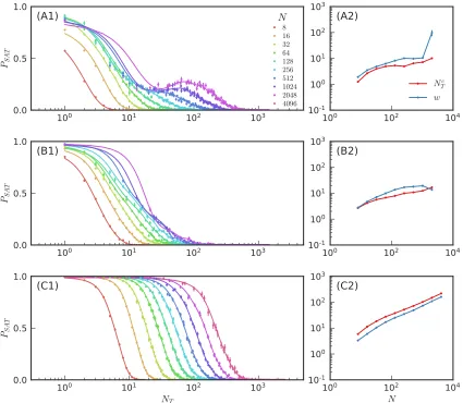
3.2 Constraint satisfaction phase transition statistics . . . 52
3.3 Number of removed edges for multifunctional networks . . . 54
3.4 CSP transition for different sources . . . 73
3.6 CSP transition for mechanical networks with different target response
magnitudes . . . 75
3.7 CSP transition for different node connectivities . . . 76
3.8 CSP transition for triangular lattices . . . 76
3.9 CSP transition for global sources . . . 77
3.10 CSP transition for tuning current or tension . . . 78
3.11 CSP transition for flow networks with negative target responses . . . 79
3.12 CSP transition for mechanical networks with negative target responses 80 3.13 CSP transition for UK railroad networks . . . 81
3.14 CSP transition deviations from power law scaling . . . 83
4.1 Comparison of flow network structure vs. function . . . 94
4.2 Comparision of flow network structure for different tuning thresholds 95 4.3 Persistence algorithm for flow networks . . . 100
4.4 Evolution of persistence diagrams with tuning . . . 101
4.5 Persistence-based coarse-graining procedure . . . 106
4.6 Comparison of coarse-graining procedure and topological structure of two flow networks . . . 107
4.7 Evolution of flow network structure with tuning . . . 110
4.8 Effective pressure difference of flow network sectors vs. tuning threshold112 4.9 Persistence of flow network sectors . . . 113
4.10 Properties of flow network sectors . . . 116
4.11 Topological structure of multifunctional flow network . . . 119
A.1 Model for stress propagation in the myocardium . . . 149
A.5 FEM “cell-on-gel” model . . . 180
A.6 Comparison of point-like and finite-sized cardiomyocytes . . . 181
A.7 Measurements of heart tissue viscoelastic response . . . 185
A.8 Adult heart BPM with and without conduction interference drugs . . 186
A.9 Embryonic heart characterization with and without conduction inter-ference drugs . . . 187
A.10 Blebbistatin interference of embryonic heart . . . 188
A.11 Blebbistatin interference and rescue of embryonic heart . . . 189
A.12 Video of chick hearts pre- and post-onset of beating . . . 190
A.13 Video of adult mouse hearts pre- and post-conduction interference . . 191
Chapter 1
Introduction
The term allostery was originally coined in 1961 by Monod and Jacob [46] to
de-scribe the inhibition of proteins “where the inhibitor is not a steric analogue of the
substrate [8].” Accordingly, it is composed of two Greek roots: allos, meaning “other”
or “different” and stereos, meaning “solid” or “body”, signifying the “difference in
specificity of the two binding sites for regulatory effector and for substrate [8].” Since
its conception, allostery has become a central focus in molecular biology, arriving
at its modern definition as “the process by which biological macromolecules (mostly
proteins) transmit the effect of binding at one site to another, often distal, functional
site, allowing for regulation of activity [47].”
the structural complexity inherent to proteins, poses a significant barrier towards
de-veloping a theoretical model that generally applies to all proteins. Faced with this
apparent disconnect between protein structure and function, much effort has instead
concentrated on developing methods to characterize allosteric mechanisms in
individ-ual proteins. These methods often focus on quantifying the dynamic and structural
conformational changes undergone by allosteric proteins or identifying pathways of
residues responsible for communicating allosteric signals [59, 14]. The guiding hope
behind this approach is that understanding the allosteric mechanisms of enough
in-dividual proteins will help to identify generic motifs, eventually providing enough
insight to develop a unified conceptual description.
Over the last few decades, a common perspective has arisen that allostery is a property
of a protein’s underlying network of interactions. In many of the approaches that have
been developed to characterize allostery, a protein is approximated as a mechanical
(or elastic) network, with edges (bonds) representing interactions between amino
acids [35]. When a localized source is applied at one site, the signal is mediated by
the network to induce a specific localized response at a second distant site. Although
this phenomenon has historically been discussed in the context of proteins, allostery
has also been more broadly framed as a property of any molecular system composed
of a network of interactions [14]. Here we propose an even more inclusive definition
of allostery: it is not just a property of molecules, but rather a property of complex
networks in general. Given this broader definition, many other types of naturally
In particular, venation networks in animals [77], plants [55, 66], fungi [33], and slime
molds [74] present an interesting example, as they are often composed of complex
hier-archical network structures that are optimized to direct flow from a limited number of
inputs to support local activity or growth throughout the system. While much effort
has been devoted to understanding the design and optimization of general transport
networks [1], the problem of fuctional control in flow networks has never been framed
in the context of allostery. This is in spite of the close mathematical relationship
be-tween mechanical and flow networks; in the linear regime, flow (or resistor) networks
can be mapped onto one-dimensional linear spring networks [73]. This correspondence
provides an alternative framework within which to study allostery, as flow networks
are less mathematically complex (having less degrees of freedom per node), but still
share many of the qualitative behaviors of their higher-dimensional counterparts.
Ex-perimental studies of biological flow networks suffer from some of the same obstacles
encountered when studying proteins. This is especially apparent in systems such as
the brain vasculature where significant variation in micro-scale architectures can exist
between individuals [32], although brains from individuals within the same species (or
even between different species) are ostensibly able to redistribute blood in the same
ways. Understanding how this variation does or does not affect function is difficult
as experiments are limited to sampling network architectures from relatively small
numbers of – or even single – individuals [13].
occurs over many generations via the accumulation of genetic mutations, modifying
a protein’s constituent amino acids and consequently its network of interactions. If
these changes cause the protein to develop some beneficial allosteric functionality,
then the corresponding genes may experience positive selection. On the other hand,
many venation networks can actively redirect flow as dictated by the needs of the
system. For example, the cerebral vasculature can dynamically contract and dilate
blood vessels, enabling the brain to actively control the propagation of blood to
support local neuronal activity [29, 26]. More generally, the ability to locally tune
the conductances of individual vessels in venation networks enable animals, fungi,
and slime molds to control the spatial distribution of water, nutrients, oxygen, or
metabolic byproducts.
Taking inspiration from the ability of both proteins and venation networks to
modu-late functionality, this dissertation follows an alternative route towards developing an
understanding of allostery. We approach allostery from the perspective of
metamate-rials design, developing techniques to create synthetic allosteric networks in both flow
and mechanical systems. In mechanical networks, we define allostery in terms of the
elastic response to applied strains, while in flow networks we consider the
redistribu-tion of pressures upon the applicaredistribu-tion of external pressure sources. In both cases, an
allosteric function is one in which a specific target site responds in a predetermined
way when a source is applied at a predetermined site elsewhere in the network.
Not only does designing synthetic allosteric systems allow us to determine the
of such networks. By using these ensembles, we are better able to investigate the
types of allosteric function that are possible and simultaneously reveal the seemingly
complex relationship between structuture and function. We can also investigate to
what extent allosteric mechanisms are optimal and the trade-offs between this
opti-mality and adaptability. By efficiently creating synthetic allosteric networks, we can
also better study the statistical variation in the network architectures of such systems
without the constraints imposed by limited experimental data. The inclusion of flow
networks in our studies helps to generalize our results, providing a system which is
often simpler to understand while still giving us insight in mechanical systems.
This thesis contains content that is primarily reproduced in order from Refs. [61],
[62], and [63]. Chapter 2 starts by presenting methods to create synthetic allosteric
mechanical networks in both theory and experiment. We find that creating allosteric
functionality is remarkably easy; by simply removing a small percentage of the bonds
in a spring network, almost any initial network can be tuned to exhibit allosteric
behavior. This shows that the requirements of allostery are minimal, simply
ne-cessitating a network to have enough tunable degrees of freedom. Next, Chapter 3
extends the tuning method to include flow networks. Using this combined
frame-work, we show that the limits of multifunctionality in both systems are set by the
same constraint satisfaction phase transition. This provides strong evidence that the
problems of controlling allosteric behavior in flow and mechanical networks belong
the relationship between structure and function is topological in nature, providing a
universal characterization that applies to all tuned allosteric flow networks.
An additional supplemental chapter is provided at the end of the thesis, reproducing
content from Ref. [6]. This chapter contains work to which I contributed
signifi-cantly at the beginning of my doctoral studies, but does not fit as cleanly into the
narrative of this dissertation outlined above. In this work, we developed a model
of the embryonic chicken heart as a mechanically active medium. When the heart
beats, cardiac muscle cells contract in a coordinated fashion, generating a nonlinear
contractile wavefront that propagates across the heart. Traditional models of this
behavior assume this wavefront is coordinated via electrical signaling between cells.
However, recent experiments revealed that the velocity of this wavefront can depend
on the mechanical properties of the cardiac tissue, behavior that cannot be explained
by standard electrochemical signaling. To remedy this, we proposed a mechanical
signaling mechanism in which cells contract in response to strains exerted by their
neighbors. Our prediction that the embryonic heart would continue to beat even in
the absence of electrical signaling was confirmed experimentally using gap junction
blocking drugs. This result demonstrated that the embryonic heart does indeed use
mechanical signaling to coordinate the heartbeat. While this work is not
specifi-cally concerned with allostery in biological networks, it still adheres to the theme of
long-range signaling in complex biological systems. By utilizing a mechanical
signal-ing mechanism, the embryonic heart is able to robustly propagate mechanical strains
If one desired, this long-range signaling behavior could be interpreted as a dynamic
form of allostery, further demonstrating that developing a general understanding of
Chapter 2
Designing allotery-inspired
response in mechanical networks
Note: The following content is reproduced with minor revision from Ref. [61].
2.1
Introduction
The ability to tune the response of mechanical networks has significant applications
for designing meta-materials with unique properties. For example, the ratio G/B
of the shear modulus G to the bulk modulus B can be tuned by over 16 orders
of magnitude by removing only 2% of the bonds in an ideal spring network [28].
Such a pruning procedure allows one to create a network that has a Poisson ratio
ν anywhere between the auxetic limit (ν = −1) and the incompressible limit (ν =
a network controls the width of a failure zone under compression or extension [15].
Both these results are specific to tuning the global responses of a material. However,
many applications rely on targeting a local response to a local perturbation applied
some distance away. For example, allostery in a protein is the process by which a
molecule binding locally to one site affects the activity at a second distant site [59].
Often this process involves the coupling of conformational changes between the two
sites [11]. Here we ask whether disordered networks, which generically do not exhibit
this behavior, can be tuned to develop a specific allostery-inspired structural response
by pruning bonds.
We introduce a formalism for calculating how each bond contributes to the mechanical
response anywhere in the network to an arbitrary applied source strain. This allows
us to develop algorithms to control how the strain between an arbitrarily chosen pair
of target nodes responds to the strain applied between an arbitrary pair of source
nodes. In the simplest case, bonds are removed sequentially until the desired target
strain is reached. For almost all of the initial networks studied, only a small fraction
of the bonds need to be removed in order to achieve success. As was the case in
tuning the bulk and shear moduli, we can achieve the desired response in a number
of ways by pruning different bonds. We have extended our approach to manipulate
multiple targets simultaneously from a single source, as well as to create independent
responses to different locally applied strains in the same network. Our central result
We demonstrate the success of this method by reproducing our theoretical networks
in macroscopic physical systems constructed in two dimensions by laser cutting a
planar sheet and in three dimensions by using 3D printing technology. Thus, we
have created a new class of mechanical meta-materials with specific allostery-inspired
functions.
2.2
Theoretical Approach
Our networks are generated from random configurations of soft spheres in three
di-mensions or discs in two didi-mensions with periodic boundary conditions that have
been brought to a local energy minimum using standard jamming algorithms [51, 43];
the spheres overlap and are in mechanical equilibrium. We convert a jammed packing
into a spring network by joining the centers of each pair of overlapping particles with
an unstretched central-force spring. We chose this ensemble because it is disordered
and provides initial networks with properties – such as elastic moduli – that depend
on the coordination of the network in ways that are understood [19, 20, 28]. We can
work either with the entire system that is periodically continued in space or with a
finite region with free boundaries that is cut from the initial network.
Starting with a network with N nodes and Nb bonds in d dimensions, our aim is to
tune the strain εT between a pair of target nodes in response to the strain εS applied
chosen so that they are not initially connected by a bond; see Appendix). We create
a specific response in our system by tuning the strain ratio η = εT/εS to a desired
valueη∗. At each step, we calculate to linear order the change inη in response to the
removal of each bond in the network using a computationally-efficient linear algebra
approach (see Methods). We then remove the bond which minimizes the difference
between η and η∗ and repeat until we reach a desired tolerance.
2.3
Computational Results
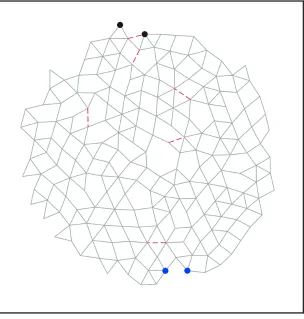
(A)
Target
Source
(B)
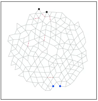
Figure 2.1: Network with 194 nodes, 407 bonds at ∆Z = 0.19 tuned to exhibit (A) expanding (η = +1) and (B) contracting (η = −1) responses to within 1% of the desired response. Source nodes are shown in blue, while target nodes are shown in black. Arrows indicate the sign and magnitude of the extension between the pairs of source and target nodes. The removed bonds are shown as red lines.
We apply our tuning approach to networks with free boundaries in both two and
for rigidity in a network with free boundary conditions [27]. For each trial, a pair
of source nodes was chosen randomly on the network’s surface, along with a pair of
target nodes located on the surface at the opposing pole. (Note that we could have
chosen anywhere in the network for the location of the source and target.) In two
dimensions we chose networks that on average had 190 nodes and 400 bonds before
tuning, with ∆Z ≈0.19. In three dimensions networks had on average 240 nodes, 740
bonds and ∆Z ≈0.18. Prior to pruning, the average strain ratio of the networks in
two dimensions wasη≈0.03 and in three dimensions wasη≈0.2 for the system sizes
and ∆Z values we studied. The response of each network was tuned by sequentially
removing bonds until the difference between the actual and desired strain ratios, η
and η∗ respectively, was less than 1%.
To demonstrate the ability of our approach to tune the response, we show results
for η = ±1. Note that η > 0 (< 0) corresponds to a larger (smaller) separation
between the target nodes when the source nodes are pulled apart. Fig. 2.1 shows a
typical result for a two-dimensional network: in Fig. 2.1(A), the strain ratio has been
tuned toη = +1 with just 6 (out of 407) bonds removed; Fig. 2.1(B) shows the same
network tuned to η = −1 with a different set of 6 removed bonds. The red lines in
each figure indicate the bonds that were pruned. Animations of the full nonlinear
responses of these networks are provided in Videos 2.8 and 2.9 of the Appendix. We
note that some of the removed bonds are the same for both η= +1 and η=−1.
The average strain ratio versus the number of removed bonds is shown in Fig. 2.2(A).
0
2
4
6
N
r
®-4.0
-2.0
0.0
2.0
4.0
η
(A)
10
-110
010
110
2|
η
|
0.00
0.05
0.10
0.15
0.20
Failure Rate
(B)
0
5
10
15
20
N
r
0.0
0.1
0.2
0.3
0.4
0.5
Probability
0
1
2
3
4
N
r
/
N
r
®0.0
0.4
0.8
1.2
N
r
®P
(
N
r
)
(C)
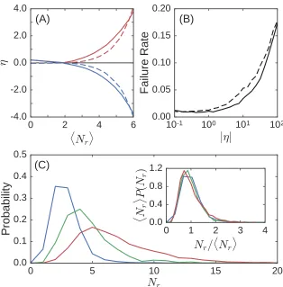
Figure 2.2: (A) Strain ratioη versus the number of removed bonds Nr for expanding
(red) and contracting (blue) responses in both 2D (solid lines) and 3D (dashed lines). For each response type and dimension, the strain ratio is averaged over 1024 tuned networks constructed from 512 initial systems. Networks in 2D have about 190 nodes and 400 bonds on average with an initial excess bond coordination of ∆Z ≈ 0.19, while those in 3D have about 240 nodes and 740 bonds on average with ∆Z ≈0.18. (B) Failure rate of tuning systems to within 1% of a specified strain ratio magnitude in 2D (dashed lines) and 3D (solid lines) averaged over contracting and expanding responses. (C) The distribution of the number of removed bonds for three different strain ratio magnitudes: |η| = 0.1 (blue), |η| = 1.0 (green), and |η| = 10.0 (red). Inset: All three distributions collapse when scaled by the average number of removed bonds hNri.
In two dimensions only about 5 bonds out of about 400 were removed on average
(∼1%); similarly, in three dimensions only about 4 bonds out of about 740 were
than 2% for strain ratios of up to |η| = 1 in two dimensions and less than 1% in
three dimensions. Therefore, not only does our algorithm allow for precise control of
the response, it also works the vast majority of the time. The failure rate increases
significantly for |η| 1, but here we are considering only the linear response of the
network. Extremely large values of η necessitate an extremely small input strain at
the source and may therefore not be physically relevant.
The failure rate is insensitive to ∆Z except at very small values. In the small ∆Z
regime the failure rate is higher because very few bonds can be removed without
compromising the rigidity of the system. If we increase the bond connectivity to
∆Z ≈ 1.0 for networks in two dimensions, the failure rate remains very low, but
bonds are removed in a thin region connecting the target and source. This narrowing
of the “damage” region is reminiscent of the results of Ref. [15], in which bonds above
a threshold stress were broken, or of Ref. [28], in which bonds that contribute the
most to either the bulk or shear modulus were successively pruned.
Fig. 2.2(C) shows the distribution of the number of bonds that must be removed to
tune a network to within 1% of a desired strain ratio for |η|= 0.1, 1, and 10. These
distributions are broad and the mean shifts upwards as η increases. The inset shows
that the distributions collapse when normalized by the average number of removed
bonds hNri. Note that we do not achieve the desired strain ratio simply by tuning
the entire free surface of the network to have large strain ratios; the response of the
designated target is large while the response between other pairs of nodes is essentially
10
-310
-210
-110
010
1|η|
10
-410
-210
010
2Probability
Figure 2.3: Distribution of strain ratios for pairs of neighboring nodes on the surface (excluding the source and target pairs) of the networks before (red) and after (blue) tuning. Results are shown for 2D networks that had on average 190 nodes and 400 bonds with ∆Z ≈0.19. This includes 512 initial networks each tuned separately to a positive and negative strain ratio with magnitude |η|= 1.0 for a total of 1024 tuned networks. Tuned networks are only included if the tuned strain ratio is within 1% of the desired strain ratio. The response for pairs other than the source and target are essentially unaffected. The target strain ratio is shown with a vertical dashed line. All distributions include both contracting and expanding responses.
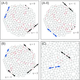
Fig. 2.4 demonstrates the variety of responses that we are able to create. Fig. 2.4
3(A-I) and (A-I3(A-I) show a single network with two independent sources and targets whose
responses were tuned simultaneously and independently of one another. When a
strain is applied to the first pair of source nodes, its target responds strongly while
the other target does not respond at all. Likewise, when the strain is applied to the
second pair of source nodes, its target responds while the first target does not. In
Fig. 2.4(B), a network with one pair of source nodes controls three targets, each of
which has been tuned to a different strain ratio. These networks have ∆Z = 1.0;
the failure rate for creating these more complicated responses is generally higher for
η
=
−1
η
= 2
η
= 1
(B)
η
=
−1
η
= 0
(A-I)
η
= 0
η
=
−1
(A-II)
(C)
Figure 2.4: (A) Network with 200 nodes and 502 bonds at ∆Z = 1.0 with two inde-pendent responses tuned simultaneously into the system. (A-I) One target contracts in response to a strain at the first pair of source nodes while the other target does not respond. (A-II) Second target responds to a strain at the second source while the first target remains unaffected. This demonstrates that separate responses can be shielded effectively from one another. (B) Same network tuned to show responses at three targets with responses of η = 1, 2, and −1. All three targets are controlled by a single pair of source nodes. (C) Periodic network with 254 nodes and 568 bonds at ∆Z = 0.47 tuned to display an expanding response with η= 1, showing that open boundaries are not necessary for tuning to be successful.
without free boundaries (see Video 2.10 in the Appendix for an animation of the
nonlinear response). We have also found that initial disorder in the network is not
necessary for success (Fig. 2.5(A)), nor is close proximity of the two nodes comprising
(A)
(B)
Figure 2.5: (A) Periodic triangular lattice with 256 nodes and 768 bonds at ∆Z = 2.0 tuned to exhibit a strain ratio of η = 1.0. This example shows that disorder in the initial network is not necessary for a response to be tuned successfully. (B) Network with 200 nodes and 457 bonds with ∆Z = 0.57 tuned to show a strain ratio ofη= 1.0. This demonstrates that the proximity of the source nodes to each other, and similarly the target nodes, is also not necessary for success.
2.4
Experimental Results
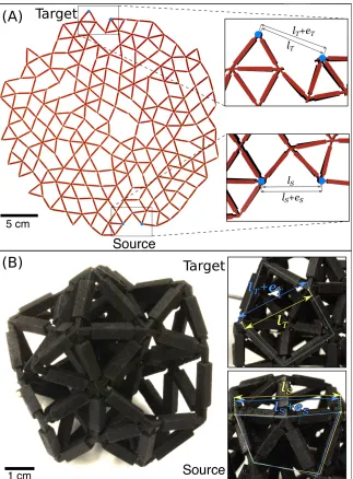
Fig. 2.5(A) shows an image of a two-dimensional network created by laser cutting a flat
sheet. The network is the same as the simulation shown in Fig. 2.1(A). The
zoomed-in areas show the strazoomed-in response at the target along with the applied strazoomed-in at the
source nodes. Video 2.11 of the Appendix shows the response of a similarly designed
network. Fig. 2.6(B) shows an image of a three-dimensional network created by 3D
printing. In this case, the network was designed to have a strain ratio ofη=−5. The
insets again show the relative strains between the pairs of target and source nodes.
In order to obtain a quantitative analysis of how well the physical realizations agree
two-Figure 2.6: (A) Physical realization of the network in Fig. 2.1(A). The zoomed-in photographs show the initial and final distance between the pair of source nodes, lS
and lS+eS, respectively, and between the pair of target nodes, lT and lT +eT. The
undeformed network is shown in black, while the deformed network is superimposed in red. (B) Photograph of a three-dimensional network constructed by 3D printing with 33 nodes and 106 bonds at ∆Z = 0.42 tuned to exhibit a negative response (η = −5.0). In the zoomed-in photographs, the yellow and blue arrows show the distance between the undeformed, lS (lT), and deformed, lS +eS (lT +eT), source
(target) nodes, respectively.
ity of the bonds do not change their length appreciably. We therefore focus only on
network was tuned. As one might expect, these are the most sensitive to the applied
source strain. We calculate, for those changes in distances, the Pearson correlation
coefficient between the experiments and the simulations:
C = h(xi− hxii)(ci− hcii)i σxσc
(2.4.1)
Herexi (ci) is defined as the fractional change due to the source strain in the distance
between nodes initially connected by bond i as measured in experiments (computer
simulations). The standard deviations ofxi andciareσxandσc, respectively. We find
that when averaged over 4 experimental realizations of different designed networks,
C = 0.98±0.02. This indicates that the experiments are very accurate realizations
of the theoretical models.
In contrast to our simulations, where junctions are connected only via central-force
springs, our experimental systems have physical struts between the nodes. This
in-troduces bond-bending forces because the struts emerging from a node have preferred
angles between them. In order to minimize such forces, we have manufactured the
struts with a non-uniform width so that they are thinner at their ends where they
attach to a node than along the rest of their length. This ensures that the struts
deform preferentially near the nodes rather than buckling in their middle. Figure 5
shows that decreasing the width of the thinnest part of the struts alleviates effects
Apart from bond-bending, there is also a possibility of two-dimensional networks
buckling out of the plane, along with nonlinear effects that are present in real systems
undergoing finite strains. All these factors can weaken the designed response. To
investigate these effects, we used laser cutting to create realizations of 10 of the
two-dimensional networks produced from the computations in Fig. 2.2. The networks
chosen were tuned successfully in the linear regime and had nonlinear responses within
a factor of two of the linear prediction at a source strain of 5%, according to our
computations. For the experimental realizations, we found that in the nonlinear
regime, 3 of the networks demonstrated a response that was more than 10% of the
designed response at a source strain of 5%.
1.00
1.25
1.50
1.75
2.00
w
[mm]
0.1
0.2
0.3
0.4
0.5
η
2 mm
w
2.5
Discussion
We have shown that it is strikingly easy to tune allosteric deformation responses into
an arbitrary spring network by removing only a small fraction of the bonds. Not
only can we tune the strain ratio to large negative or positive values for the same
network, but we achieve strain ratios of order |η| ∼ 1 with almost 100% success.
Our theoretical approach can also be extended to more general responses. We can
control multiple pairs of target nodes simultaneously with the same pair of source
nodes and we can tune multiple independent source/target responses simultaneously
into a network. We have also achieved similarly excellent results for tuning responses
in periodically-continued systems.
The approach we have described here performs a discrete optimization of the
re-sponse. We have also tuned the response using a standard numerical optimization
technique (e.g., gradient descent), by varying the stiffnesses of all the bonds
contin-uously. This brute-force method is less efficient but equally successful in producing
a desired response, and has the advantage of being able to tune nonlinear behavior.
Our approach can also be generalized to other types of bond manipulation such as
introducing new bonds.
Our theoretical approach provides a framework for understanding and controlling the
In addition, our theoretical approach can be generalized to other problems such as
origami, where one may wish to tune the fold structure so that the system folds in
a specific way in response to locally applied external forces [24]. This problem is
similar to ours, except that folds are added instead of bonds being removed. Ref. [24]
introduces an optimization technique in which fold rigidities vary continuously. This
technique is computationally expensive because the network response must be
recal-culated with each optimization step. A generalization of our theoretical approach to
origami, using language similar to that of Ref. [67], could lead to a more efficient
algorithm.
The network responses we create are reminiscent of the localized, long-range-correlated
deformations which characterize allostery in proteins. In fact, folded proteins have
long been modeled as elastic networks [35] and the response to localized forces in the
resulting networks has been studied [2]. Our results demonstrate the ease with which
allosteric conformational changes in networks can be achieved by removing a very
small set of bonds. As such, it suggests why allostery is so common in large biological
molecules [31].
Similarly, our finding that networks can be tuned to have a variety of different
re-sponses may help elucidate multifunctional behavior [49] and multiple allosterically
interacting sites [84] in proteins. It has also been observed that small changes in a
protein’s covalent structure can often change its biochemical function [37]. One might
ask whether our method could be extended to develop a systematic way to determine
been emphasized that the ability to control allosteric responses in folded proteins
could lead to significant advances in drug design [50, 30]. While much work has
fo-cused on identifying, understanding and controlling pre-existing allosteric properties,
the question of how to introduce new allosteric functions is relatively unexplored [14].
Our success in constructing experimental systems in spite of nonlinear and
bond-bending effects suggests that results are often robust even outside the simple linear
regime. However, proteins are thermal whereas our networks are athermal
struc-tures. Statistical fluctuations in the structure of proteins has been shown to play an
important role in allosteric functionality [76, 47]. In the linear response regime, the
equilibrium response at finite temperature is equivalent to that at zero-temperature,
so the set of bonds that are removed and the average strain ratio are independent
of temperature in the harmonic regime. However, the nonlinear response will show
differences, particularly at temperatures beyond the harmonic regime. It is thus
im-portant to investigate how thermal effects can influence the ability to design a desired
response in the nonlinear regime. In addition, protein contact networks generally
con-tain pre-stressed bonds, as well as bond-bending and twisting constraints, while our
theoretical networks are constructed in the absence of such effects [18, 75, 71].
Further work needs to be done to understand why removing specific bonds achieves
the desired response. Our method of identifying the elements of the stress basis
including the number of targets that can be controlled and the number of
indepen-dent responses that can be tuned for networks of a given size and coordination. To
understand experimental systems ranging from proteins to the macroscopic networks
we have fabricated, we must extend the theory to include temperature, dynamics,
pre-stress, bond-bending, and nonlinear effects due to finite strains. Our approach
provides a starting point for addressing these issues.
2.6
Materials and Methods
2.6.1
Computed Networks and Choice of Source and Target
Nodes
To create a finite network, we choose a cut-off radius from the center of our box
and remove all bonds that cross that surface. This process often creates zero energy
modes at the boundary of our network. Since we require rigid networks, we remove
nodes associated with these modes. We calculate zero modes by performing a spectral
decomposition of the dynamical matrix. For each zero mode calculated this way, we
identify the node with the largest displacement amplitude and remove it. We then
recalculate the zero modes and repeat this process until no zero modes exist. This
method of removing zero modes works in any dimension and does not require an
arbitrary threshold for whether a node contributes to a zero mode or not. Our final
dimensions with N nodes andNb bonds.
We choose the pair of source nodes to lie on the exposed surface of the networks.
The pair of target nodes is chosen to be on the opposing pole of the network surface.
When choosing a pair of nodes, we also ensure that they are not connected by a bond.
This is done to avoid surface bonds whose tensions do not couple the the rest of the
network. However, since our formalism relies on applying tensions and measuring the
strains of bonds, we introduce a bond of zero stiffness, called a “ghost” bond, between
each pair of nodes for convenience (see Appendix).
2.6.2
Further Details of Theoretical Approach
Our approach tunes the ratioη=εT/εS of the target strainεT to the source strainεS
by removing bonds sequentially, one at a time. First, we define the cost function which
measures the difference between the network’s response η and the desired response
η∗. This is given by
∆2 ≡
n
X
j=1
(ηj/ηj∗−1)2 if η∗j 6= 0
η2
j if η∗j = 0
(2.6.1)
where j indexes the targets and their corresponding sources (e.g., n = 1,2,3 in
to remove the bond which creates the largest decrease in ∆2.
To decide which bond to remove, we must calculate how the removal of each bond
changes η. First we define the vectors of bond extensions |ei and bond tensions |ti
in response to the externally applied strain, each of length Nb. In order to access
the extensions and tensions on individual bonds, we define the complete orthonormal
bond basis |iiwhereiindexes the bonds. The extension on bondican then be found,
ei = hi|ei, along with the bond tension, ti = hi|ti. The strain of bond i is εi =ei/li
whereli is the bond’s equilibrium length. The tension and extension are related by a
form of Hooke’s law,
|ti=F−1|ei (2.6.2)
where the flexibility matrix is defined as hi|F|ji=δij/ki. Here we choose the stiffness
of bondito beki =λi/liwhereλi is the bond’s material modulus with units of energy
per unit length.
In addition to the bond tensions and extensions, we can define the dN-vectors of
node displacements |ui and net forces on nodes |fi. The equilibrium matrix Q
relates quantities defined on the bonds to those defined on the nodes through the
expressions QT |ui = |ei and Q|ti = |fi [7]. In general Q, is a rectangular matrix
with dN rows and Nb columns. The total energy can then be written
E = 1
where the Hessian matrixH =QF−1QT is a dN ×dN matrix. In the presence of an
externally applied set of tensions |t∗i, the minimum energy configuration satisfies
H|ui=Q|t∗i. (2.6.4)
To calculate the change in the displacements if a bond were removed, the naive
approach would be to set the stiffness to zero for that bond in the flexibility matrix and
to solve this equation. However, performing this matrix inversion to test the removal
of each bond can be prohibitively expensive with a computational cost of O(NbN3),
so we have developed a more efficient approach. Note that here we calculate the
response to applied tensions, not the strains we need to calculate η. However, since
we are only interested in the ratio of the target strain to the source strain and are
working in the linear regime, we do not need to explicitly apply a strain nor specify
the tension amplitude.
We use the equilibrium matrix Q to define a convenient basis of the bond tensions
and extensions. Performing a singular value decomposition of Q gives access to is
right singular vectors [54]. This yields two mutually orthonormal sub-bases of vectors
that together form a complete basis of size Nb. The first sub-basis is comprised of
vectors with singular values of Qthat are zero; that is, tensions that do not result in
net forces on the nodes. These are commonly known as thestates of self-stress (SSS),
correspond to valid displacements. The second sub-basis is comprised of vectors with
positive singular values of Q; tensions that correspond to net forces on nodes, or
extensions that are compatible with node displacement. We call these vectors the
states of compatible stress (SCS) and denote them as |cαiwhereαindicates the basis
vector. In total there are Nc SCS basis vectors and Ns SSS basis vectors which total
toNc+Ns =Nb.
Using these two sub-bases (and rescaling the bond stiffnesses so they are identicallk;
see Appendix), we can calculate the discrete Green’s function
G= 1 k
X
α
|cαi hcα| (2.6.5)
which maps bond tensions to extensions. Using this result, we calculate the change
in the bond extension vector |eiif bond i were to be removed,
|∆ei= |Cii h
Ci|t∗i
k(1−C2
i)
(2.6.6)
where |Cii = kG|ii and Ci2 ≡ hCi|Cii. From this equation we can calculate the
changes in bothεT andεS and therefore the changeη. This result can also be derived
by inverting (2.6.4) and using the Sherman-Morrison formula to calculate the change
in the inverse of the Hessian [70]. Note that this calculation does not include the zero
stiffnesses of the ghost bonds, which cannot be mapped to unity with the rest of the
system. A generalization of (2.6.6) is needed in order to take this into account (see
The next step is to calculate (2.6.6) (or its generalization found in the Appendix)
for the removal of each bond. We choose the bond which minimizes ∆2 in (2.6.1)
upon removal. One restriction is that we do not choose bonds which introduce zero
modes (see Appendix). Finally, once a bond is chosen, we recalculate the SCS and
SSS sub-bases with the bond removed (see Appendix).
A summary of our tuning algorithm contains the following steps:
1. Transform to a system where all bonds initially have the same stiffnesses and
add a ghost bond of zero stiffness for each pair of target and source nodes (see
Appendix).
2. Use the equilibrium matrix to calculate the initial SCS and SSS bases.
3. Calculate the initial extensions of the source and target bonds in response to
the applied tension t∗ using (2.6.5). Use this result to calculate the initial η.
4. For each bond, use the general form of (2.6.6) found in Eq. 2.7.15 of the
Ap-pendix to calculate the change in η if that bond were to be removed.
5. Remove the bond that minimizes ∆2 in (2.6.1). Recalculate the SCS and SSS
sub-bases with the bond removed.
We repeat steps (3) - (5) until √∆2 < 0.01 or the process fails. The computational
There are three potential sources of failure represented in Fig. 2(B): √∆2 cannot be
lowered below 0.01 by removing any bond, no bonds can be removed without creating
zero modes, or the numerical error in ∆2 exceeds 0.01. This third source of failure
arises because numerical error is introduced as bonds are removed. In order to ensure
that our results are accurate, we compare ∆2 to the value obtained from the solution
of (2.6.4) with the given set of pruned bonds removed. If the absolute value of the
difference exceeds 1%, we call it a failure. Our results constitute an upper bound on
the failure rate, which could potentially be reduced by using more accurate techniques
to decrease numerical error or more sophisticated minimization algorithms.
2.6.3
Experimental Networks
We create experimental realizations of the theoretically-designed networks in both two
and three dimensions. To make two-dimensional networks, we obtain the positions
of the nodes and struts from our design algorithm. Next, we laser cut the shape of
the network from a silicone rubber sheet. To reduce out-of-plane buckling, we use 1.6
mm thick polysiloxane sheets with a Shore value of A90. The ratio of strut length to
width within the plane of the network is approximately 10:1. The struts are designed
to be thinner at their ends in order to alleviate bond-bending.
To make three-dimensional networks, we determine the positions of nodes and struts
from the computer simulations and fabricate the networks using 3D printing
ther-moplastic elastomers) and rigid plastic (simulating acrylonitrile butadiene styrene,
ABS) with a Shore value of A85. The dimensions of each strut have a ratio of
ap-proximately 1:1:11. As in our two-dimensional networks, the struts are made thinner
at their ends.
2.7
Appendix
2.7.1
Ghost bonds
On the surface of our networks there are many nodes with exactly d bonds in d
dimensions. Any bond attached to one of these nodes is uncoupled from the rest of
the network - applying a tension to one of these bonds does not affect any tensions
or extensions on any of the other bonds in the network to linear order. Likewise, no
extensions can be measured on these bonds when a tension is applied elsewhere in
the network. Therefore, we avoid choosing pairs of source or target nodes that are
connected by uncoupled bonds. This is done by ensuring that neither the pair of
nodes comprising the source nor the target share a bond.
However, all calculations involve the bonds, so in order to apply a tension or measure
an extension between two nodes, it is convenient if they share a bond. To apply our
any direct reference to the nodes.
2.7.2
Creating identical bond stiffnesses
In order to calculate the Green’s function in Eq. 2.6.5 in the main text, it is necessary
to work in a system where all bonds have identical stiffness. However, we do not
want to be restricted to systems that satisfy this special requirement. The bonds
in our experimental systems all have the same material modulus λi = λ, but their
equilibrium lengthsli differ, resulting in bonds with non-identical stiffnesseski =λ/li.
To handle this, we start with a system in which the bond stiffnesses are all different
and map it onto an equivalent system in which all the default bond stiffnesses are
identical. This is done by introducing a flexibility matrixF (as defined below Eq. 2.6.2
in the main text) and scaling the equilibrium matrix so that ¯Q=QF−1
2. (Note: We
can only scale out stiffnesses that are nonzero.) The energy can then be written in
terms of ¯Q:
E = 1 2u
TQ¯F¯−1Q¯Tu (2.7.1)
where the scaled flexibility matrix ¯F is proportional to the identity matrix except for
any entries that are zero. This energy is the same as that in Eq. 2.6.3 in the main
Scaled extension or tension vectors are related to the unscaled versions by
|e¯i=F−12 |ei (2.7.2)
|¯ti=F12 |ei (2.7.3)
Thus we have implicitly performed all of our calculations on the scaled system and
have converted back when calculating η.
2.7.3
Discrete Green’s function
Using the SSS and SCS sub-bases, our goal is to calculate the discrete Green’s function
shown in Eq. 2.6.5. We start by decomposing the bond tensions and extensions,
|ti=X
α
|cαi hcα|ti+
X
β
|sβi hsβ|ti (2.7.4)
|ei=X
α
|cαi hcα|ei+
X
β
|sβi hsβ|ei (2.7.5)
Now suppose we apply some external tension to the bonds, |t∗i. The part of the
external tension that projects onto the SCS basis will be balanced by tensions in the
bonds, so that hcα|ti = hcα|t∗i. Additionally, the bond extensions that project onto
the incompatible extensions, or SSS basis, should be zero because they are unphysical,
we get
X
α
|cαi hcα|t∗i+
X
β
|sβi hsβ|ti=
X
α
F−1|cαi hcα|ei (2.7.6)
If we project this equation onto the SCS vector hcα0|, we get a system ofNcequations,
hcα0|t∗i=
X
α
hcα0|F−1|cαi hcα|ei (2.7.7)
=X
α
Kα0αhcα|ei (2.7.8)
where Kα0α = hcα0|F−1|cαi is an Nc×Nc square matrix. If we invert this system of
equations to solve for the extensions, we get
hcα|ei=
X
α0
Kαα−10hcα0|t∗i (2.7.9)
The full extension is then
|ei=X
α
|cαi hcα|ei=
X
αα0
|cαiKαα−10hcα0|t∗i (2.7.10)
In general, calculating the matrix inverseKαα−10 is computationally intensive since it is
a square matrix of size Nc. To improve this, we map our system to one where all the
bond stiffnesses are identicallyk or zero as described in the previous section. Finally,
we arrive at the Green’s function in Eq. 2.6.5,
G= 1 k
X
α
2.7.4
Modifying a single bond
Using the Green’s function in (2.7.11), our goal is to find the change in |ei when the
stiffness of a given bond is modified. First we define a unique SCS basis vector for
bondi,
|Cii=kG|ii (2.7.12)
This SCS is closely related to the unique SSS defined in Ref. [72]. We rotate the
SCS basis so that one of the SCS vectors is |cµi = |Cii/
p
hCi|Cii, making sure to
re-orthonormalize the rest of the basis with respect to this unique SCS. The benefit of
this rotation is that now only the unique SCS contains a nonzero element for bondi.
Next, we introduce a separate stiffness for bondi,ki which is not necessarily identical
to the rest of the bonds. The matrix Kα0α defined in the previous section can then
be simplified to
Kα0α =
kiCi2+k(1−Ci2) if α=α0 =µ
kδαα0 otherwise
(2.7.13)
where we have defined C2
i ≡ hCi|Cii= hi|Cii. The resulting extensions are
|ei= |Cii hCi|t∗i C2
i[kiCi2 +k(1−Ci2)]
+ 1 k
X
α6=µ
with change in extensions
|∆ei= |Cii h
Ci|t∗i
k(1−C2
i)
(2.7.15)
where we have taken ki from an initial value of k to zero.
2.7.5
Modifying multiple bonds
Here we extend (2.7.15) to allow for multiple bonds that do not have identical stiffness
k. Suppose that all the bond stiffnesses are identically ki = k, except for a small
subset of bonds which we callB. We say a bondi∈ B if and only if ki 6=k. This set
includes any ghost bonds with zero stiffness, along with bonds that are being tested
for removal or modification.We typically include just three bonds in B – the source
and target ghost bonds of zero-stiffness, along with the bond tested for removal.
Our goal now is to rotate our SCS sub-basis |cαi so that as few basis vectors as
possible project onto the bonds in B. We will denote this new rotated SCS
sub-basis |˜cαi. We define a special set of basis vectors V such that α ∈ V if and only if
hi|˜cαi 6= 0 for some i∈ B. Typically, the size of B will equal the size of V. In other
words, the basis vectors in V are the only vectors with non-zero elements for the set
of bonds with non-identical stiffnesses B
In order to calculate our rotated SCS sub-basis, |c˜αi, we first find the unique SCS for
are then orthonormalized using a modified Graham-Schmidt algorithm. The result
is the set of basis vectors V described previously. The remainder of the rotated SCS
basis is found by using the modified Graham-Schmidt algorithm to orthonormalize
the original SCS basis with respect to the set of vectors V, throwing out any vectors
that are completely zeroed out. The result is our set ofNc orthonormal rotated SCS
vectors. However, it will be shown that only the vectors in V will be necessary for
our solution.
Each basis vector that is not in V has zero projection onto bonds that are in B, i.e.
if α /∈ V, then hi|˜cαi = 0 for all i ∈ B. This means that if either α /∈ V or α0 ∈ V/ ,
then |˜cαi and |c˜α0i are orthogonal over a reduced basis such that
hc˜α|
X
i
|ii hi| !
|˜cα0i= h˜cα|
X
i /∈B |ii hi|
!
|c˜α0i (2.7.16)
This new basis now gives us the means to rewriteKαα0 for α /∈ V orα0 ∈ V/ ,
Kαα0 = hcα0|F−1|cαi (2.7.17)
= hc˜α|
X
i∈B
ki|ii hi|+
X
i /∈B
k|ii hi| !
|˜cα0i (2.7.18)
=kX
i /∈B
h˜cα|ii hi|˜cα0i (2.7.19)
The total matrix is then
Kαα0 =
˜
Kαα0 if α, α0 ∈ V
kδαα0 otherwise
(2.7.21)
where we have defined the sub-matrix ˜Kαα0 = hcα0|F−1|cαiforα, α0 ∈ V. We see that
the matrix inversion problem is simplified to just inverting ˜Kαα0.
Kαα−10 =
˜
Kαα−10 if α, α0 ∈ V
1
kδαα0 otherwise
(2.7.22)
Since the size ofB is very small (in our case typically a set of size 3), calculating the
inverse of this matrix is very fast. The extension can now be represented as
|ei= X
α,α0∈V
|c˜αiK˜αα−10h˜cα0|t∗i+
X
α /∈V 1
k|c˜αi h˜cα|t
∗i (2.7.23)
The change in extension on bond i when the stiffnesses are modified is then
|∆ei= X
α,α0∈V
|c˜αi∆( ˜Kαα−10)hc˜α0|t∗i (2.7.24)
Note that the solution only depends on the basis vectors in V. This means that only